Most estuarine and coastal models use second-order difference schemes (such as
second-order staggered C-grid scheme) to approximate first-order derivative
(Blumberg and Mellor, 1987; Hadivogel et al., 1991)
![]()
where p, ![]() represent pressure and grid spacing. Such a difference
scheme was proposed by numerical modelers in early 50's as the first
generation computers came into place. Since then the computer updates rapidly
with several orders of magnitude increase in computational power. However, the
difference schemes used by most modelers now are still staying at the 50's
level (second-order schemes).
represent pressure and grid spacing. Such a difference
scheme was proposed by numerical modelers in early 50's as the first
generation computers came into place. Since then the computer updates rapidly
with several orders of magnitude increase in computational power. However, the
difference schemes used by most modelers now are still staying at the 50's
level (second-order schemes).
If we go a step further by using the fourth-order C-grid scheme (Figure 1a)
proposed by McCalpin [1994],
![]()
the truncation error is on the order of O(![]() ). Comparing (2) with
(1), the error ratio between the fourth-order and second-order schemes is
estimated by
). Comparing (2) with
(1), the error ratio between the fourth-order and second-order schemes is
estimated by
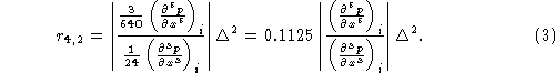
which is proportional to ![]()
Since the truncation error decreases with the increase of the order of the
difference scheme, it might be benefited to use an even higher order
difference scheme. Chu and Fan [1997] proposed a sixth-order difference scheme
![]()
![]()
to compute the horizontal pressure gradient. Comparing (4) with (1), the error
ratio between the sixth-order and second-order schemes is estimated by
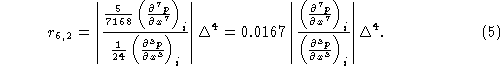
which is proportional to ![]()
There are two weaknesses of using ordinary high-order difference schemes. The
first one is more grid points needed for the computation: the ordinary 4-th
order scheme (2) needs 4 points and the ordinary 6-th order scheme (4) needs 6
points. The second one is using lower-order schemes at two boundaries. Taking
the fourth-order scheme as an example, gradient at the 'left' boundary has
second-order accuracy
![]()