
Naval
Postgraduate
School
Monterey, California
ANALYSIS OF AUV signals
by
Neil C. Rowe, Riqui Schwamm, Bruce D. Allen, and Pawel Kalinowski
February 2019
Distribution Statement A
Prepared for: Naval Research Program at NPS

Naval
Postgraduate
School
Monterey, California
ANALYSIS OF AUV signals
by
Neil C. Rowe, Riqui Schwamm, Bruce D. Allen, and Pawel Kalinowski
February 2019
Distribution Statement A
Prepared for: Naval Research Program at NPS
This page intentionally left blank
This page intentionally left blank
NAVAL POSTGRADUATE SCHOOL
Monterey, California 93943-5000
Ronald A. Route Steven R. Lerman
President Provost
The report entitled �Analysis of AUV Signals� was prepared for Navy N2/N6 and funded by NPS Naval Research Program.
Further distribution of all or part of this report is authorized.
This report was prepared by:
________________________
Neil C. Rowe
Professor of Computer Science
Reviewed by: Released by:
________________________ ______________________
Peter Denning, Chairman Jeffrey D. Paduan
Computer Science Department Dean of Research
This page intentionally left blank
We were tasked to assess the suitability of deep-learning methods for complex high-frequency signals produced by recent automated underwater vehicles. Such vehicles transmit detailed data that is considerably more complex than traditional sensors. This research is related to a recent DARPA initiative (DARPA, 2017). We interpreted the task as including several subgoals. First, we need to determine distinctive features of these signals. Second, we need to distinguish different signal sources from each other. Third, we need to distinguish periods of time within those signals and make guesses as to what is happening in each.
We were given by the sponsor three samples of AUV signals to analyze, 20 seconds each:
� The primary signal from the Griffin Aerospace MQL-110 Outlaw (1.00 gigabytes).
� The secondary signal from the Griffin Aerospace MQL-110 Outlaw (2.00 gigabytes).
� The primary signal from the Metal Shark High Speed Manueverable Surface Target (HSMST) (2.00 gigabytes).
The signal recordings were strong and had little background noise, though these issues could be important for detection and classification in many real environments (Llenas et al, 2017). Forensic analysis indicated that the data is 16-bit big-endian integers using two's complements for negative numbers, contrary to the README file. This is shown by the byte histogram having peaks for bytes having low integer values for bytes starting with a 0 bit and peaks having high integer values for bytes starting with a 1 bit, and by the much lower integer values on the average for odd-numbered bytes compared than for even-numbered bytes.
After extraction from the supplied files, raw values were found centered around 0 with a mean of 0.0067 and a standard deviation of 26.5, so the average signal value was low and this enabled clear identification of transmission periods. We obtained 500 million raw values for the Outlaw primary, 1000 million records for the Outlaw secondary, and 435.2 million for HSMST primary. If each is 20 seconds long, sampling frequencies were 25.0 mhz, 50.0 mhz, and 21.76 mhz respectively.
It should be noted that this amount of data supplied by the sponsor was inadequate for deep-learning techniques. Deep learning is a supervised kind of learning, so it requires identification of a �ground truth� or correct identifications for the data. We did not have ground truth for the periods of time in the signals. We did have ground truth about the identities of the source so we did supervised learning on that. But the first problem is the more traditional identification problem with signals.
Another obstacle to deep learning is that it requires massive amounts of data on the order of billions of examples of a concept. We just had three overall samples. We cannot just interpret the raw data points as samples because this has been shown to work poorly in many applications. A famous example illustrating this is the stop sign being consistently misinterpreted by a neural network as a �speed limit 40� sign is due to use of low-level pixel data instead of extracting the necessary concept of a �red octagon�. So we need to generalize on the raw samples in some way to get reliable and robust performance, and this is especially important for adversary signals where they will use deliberate deception to try to fool us. For raw signals, the obvious ways to generalize are the frequency patterns and the matches to various kinds of wavelets. So this is the approach we took. We can train shallower neural networks with such data, and we can test out the features that deep learning could use.
These are high-frequency signals. Analysis of such signals pose several challenges (Jondrahl et al, 1985). We are concerned with quite a bit more than just determining the modulation parameters (O�Shea et al, 2018) as we want to classify different categories of data transmission. Machine learning (Moore and Buckner, 2012) is essential to deciphering these signals as we cannot count on documentation, particularly with signals of adversaries, and we cannot depend on specialized detection tools such as Doppler radars (Mendis et al, 2017).
The interesting frequencies vary considerably for these signals. Because of this, the discrete Fourier Transform and the Fast Fourier Transform algorithms are of limited value since they find evenly spaced frequencies. We found it more helpful to convolve the signals with logarithmically spaced sine and cosine functions. Most of our experiments used 65,536-item (2 to the 16th power) segments in nonoverlapping consecutive time periods for calculation of frequency distributions. This meant the time between segments was 0.00262 seconds for the Outlaw primary, 0.00131 for the Outlaw secondary, and 0.00301 for the HSMST primary.
We used frequencies spaced by multiples of the fourth root of 2, 1.1892, ranging from a frequency corresponding to the 65,536 samples to a frequency corresponding to 2 samples. Figure 1 shows the overall frequency distributions that we observed.
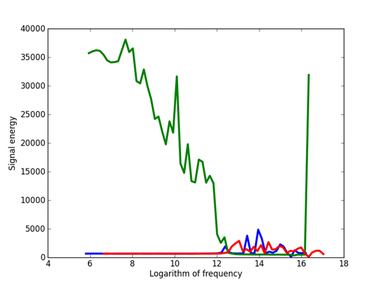
Figure 1: Frequency components observed over the three signals: Green is Outlaw primary, red is Outlaw secondary, and blue is HSMST primary.
It can be seen that the Outlaw primary is quite different from the others and its segments are easy to recognize. The jump up at the highest frequency suggests a 32-bit format, but the data were not interpretable when we tested the common 32-bit formats. However, a 32-bit format would be inconsistent with the many low frequencies observed for this signal. We suspect that this signal has some sort of run-length encoding which would account for the low frequencies, although there is no clue in the documentation. Note it could not be an encrypted signal, something mentioned in the documentation, because encryption results in a near-even frequency spectrum.
Given a set of evenly spaced time periods, a useful way to analyze the signal is to look at changes in the features of the signal over time. We computed the mean energy and standard deviation and identified time periods in which the energy was more than two standard deviations from the mean as being the likely transmission periods. We also calculated the difference in the frequency distributions between successive 65536-sample periods, a metric which can be used to detect difference in data transmission. The difference was defined by the inner product between frequency distributions. Figure 2, Figure 3, and Figure 4 show plots of the pattern of frequency differences over time. Height represents activity level and flat areas represent periods in which the frequency distribution was relatively similar and likely to represent a single transmission task. The peaks are thus likely to represent major transmissions of data. The three signals have important differences. It appears that the Outlaw primary has many irregular tasks, whereas the Outlaw secondary and the HSMST primary do many periodic transmissions.
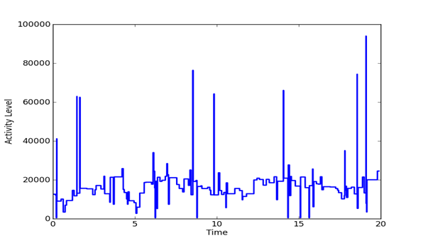
Figure 2: Changes in the frequency distribution of the Outlaw primary over the sample.
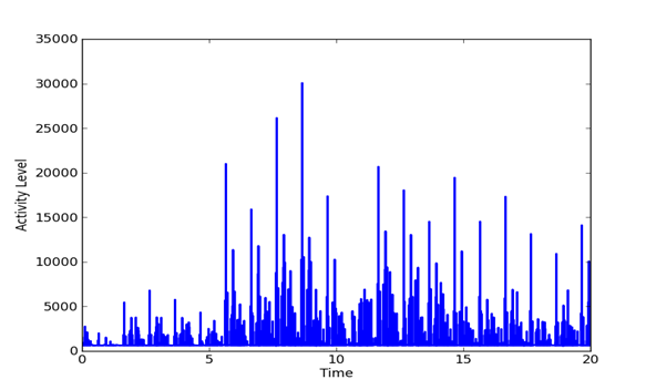
Figure 3: Changes in the frequency distribution of the Outlaw secondary over the sample.
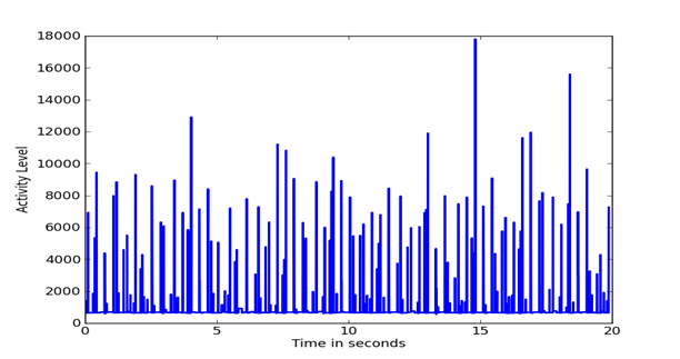
Figure 4: Changes in the frequency distribution of the HSMST primary over the sample.
Figure 5, Figure 6, and Figure 7 show details of segments of the three previous figures. It can be seen that the Outlaw secondary shows the largest amount of fine detail.
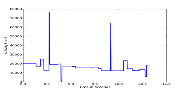
Figure 5: Details of Outlaw primary difference distributions.
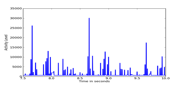
Figure 6: Details of Outlaw secondary difference distribution.
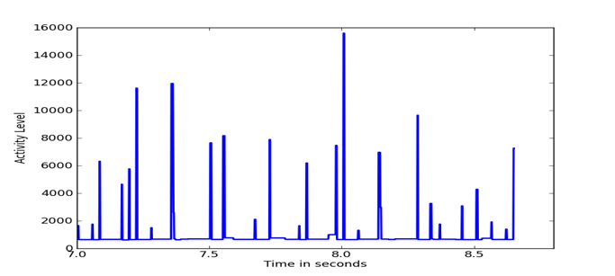
Figure 7: Details of HSMST difference distribution.
Since our signals exhibit abrupt transitions, it is useful to compute wavelet components for non-smooth wavelet families. The Haar family of wavelets are a natural choice because our signals often exhibit impulse-like behavior due to digital switching. We convolved the signals with a family of Haar wavelets at logarithmically spaced widths that were powers of 2 from 8 through 65536 and looked for local maxima. We collected all results above a threshold. We sorted the results by order of time of the center of the wavelet, and eliminated results where the width of one result period at a particular time was included in a stronger and wider result period.
Results showed there were few wide impulses in the data except for the Outlaw primary. Most strong matches were to 8-sample and 16-sample sequences, indicating frequencies for phenomena of 3-6 mhz for the 8-sample and 1.5-3 mhz for the 16-sample data.
To test ability to identify signals from their frequency distributions, we focused on 65536-sample segments, computed their components at logarithmically spaced frequencies as before, and compared them between the three signals. The cosine similarity formula is:

Comparison needed to exclude intervals in which the signaling was apparently idle and we were seeing mostly background noise. We did this by computing the root-mean squared energy for each signal every 65536 samples. Only those segments above the average energy were considered. This excluded many segments in this data.
The tables below show average similarity values and their standard deviations when 65536-sample segments are selected at random from two signals. Table 1 shows results with a sampling rate of 0.1 and Table 2 shows results with a sampling rate of 0.01 applied only the segments have more than the root-mean-square energy (a little less than half of them). The numbers are the average similarity over all segments selected, and in parentheses, the standard deviation. It can be seen that the signals are not likely to be confused except possibly the Outlaw secondary and HSMST primary.
Table 1: Similarities of frequencies of random segments of pairs of signals with 65536-sample blocks, initial sampling rate 0.1.
|
|
Outlaw primary |
Outlaw secondary |
HSMST primary |
|
Outlaw primary |
.945 (.036) |
.222 (.049) |
.072 (.079) |
|
Outlaw secondary |
.222 (.049) |
.993 (.022) |
.846 (.296) |
|
HSMST primary |
.079 (.063) |
.846 (.296) |
.943 (.036) |
Table 2: Similarities of frequencies of random segments of pairs of signals with 65536-sample blocks, sampling rate 0.01.
|
|
Outlaw primary |
Outlaw secondary |
HSMST primary |
|
Outlaw primary |
.900 (.037) |
.148 (.037) |
.079 (.063) |
|
Outlaw secondary |
.148 (.037) |
.675 (.397) |
.485 (.346) |
|
HSMST primary |
.079 (.063) |
.485 (.346) |
.973 (.108) |
We also tested with 4096-sample blocks, which gave 16 times more blocks for which 44 frequency components could be computed rather than 61 (Table 3). There were 16 times more blocks than with 35,536-sample blocks, for 122,071 blocks of Outlaw primary, 244,141 blocks of Outlaw secondary, and 106,252 blocks of HSMST primary. The 16-fold increase meant processing took 256 times longer since comparison of blocks is proportional to the product of the number of blocks. Results showed still better discrimination between signals with high rates of match of samples of similar signals. We thus recommend 4096-sample blocks for comparing high-frequency components.
Table 3: Similarities of frequencies of random segments of pairs of signals with 4096-sample blocks, sampling rate 0.01.
|
|
Outlaw primary |
Outlaw secondary |
HSMST primary |
|
Outlaw primary |
.993 (.012) |
.636 (.079) |
.176 (.131) |
|
Outlaw secondary |
.636 (.079) |
.998 (.004) |
.950 (.097) |
|
HSMST primary |
.176 (.131) |
.950 (.097) |
.997 (.009) |
We also compared signals in the time domain by convolving them with a sliding offset, select the best offset for each segment of one signal. To make sure we examined each possible offset, we used a window of 65536*2 for one signal for the window size of 65536 in the other signal. Again we excluded segment having less than the root-mean-squared energy.
With this similarity analysis, the simplest way to classify signals in the wild is by a case-based reasoning approach: We take a 65,536-element sample of the data, and compute either its frequencies or its convolutions to known signals. Then the closest match can be used to identify the signal
.
This approach is very computationally intensive. We implemented it on our Hamming/Grace supercomputer using the Apache Spark framework, using methods we have used previously for combat identification data (Rowe et al, 2018), but it still was computationally infeasible to do in full as is explained in Appendix B.
Another way to compare signals is to try to distinguish digital features within the time domain of the signals. A simple approach is to identify patterns of important changes in the energy of the signals since they exhibit many abrupt transitions from waiting to transmitting. We used the results of the wavelet analysis to count pairs of successive strong wavelet matches (bigrams), triples of success strong wavelet matches (trigrams), and quadruples (quadgrams). Those with high counts are likely good indicators of distinctive phenomena in the signal. To require a degree of simultaneity, bigrams and trigrams needed to occur within a certain window of time to suggest association; we focused on gaps of less than 4096 samples. To give a sense of the data, Figure 8 shows the distribution of the natural logarithms of gaps between the first two wavelet matches in a triple, Figure 9 shows the distribution of the lengths of the strongest spans of the wavelets, and Figure 10 shows the distribution of the differences in the strengths of the wavelets for the first two matches.
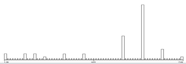
Figure 8:Natural logarithm of the gap in samples between the first two wavelet features of observed trigrams.
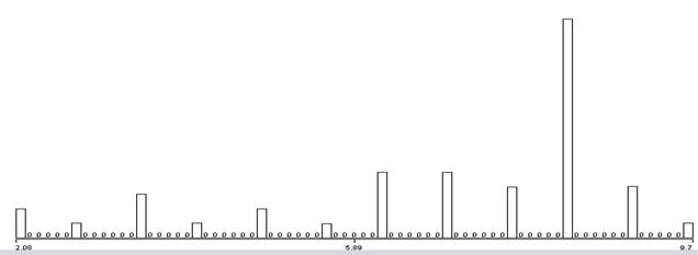
Figure 9: Natural logarithm of the length of the first wavelet match in observed trigrams.
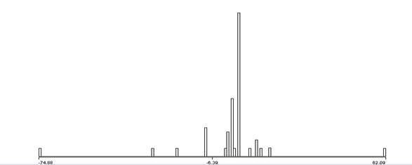
Figure 10: Difference in signed strength of wavelet matches in the first two items of trigrams.
For experiments, we set a threshold of 25 on the average absolute
value of the change in the signal energy between the first half of the wavelet
and the second half, and found the largest such change over all wavelet
spans. This threshold seemed to be the best for finding useful features
without finding too many false alarms. We found 67 bigrams, 37 trigrams,
and 15 quadgrams in the Outlaw primary; 1392 bigrams, 8379 trigrams, and 17,586
quadgrams in the Outlaw secondary; and 1876 bigrams, 5737 trigrams, and 12,278
quadgrams in the HSMST primary. The preponderant lower frequencies for
the Outlaw primary meant the n-grams found covered a considerably wider span of
time, however, and thus were more accurate features of the signal. Table
3 shows the cosine similarities of the bigrams and Table 4 shows the
similarities of the trigrams. Two numbers are given for each entry:
similarity with unweighted counts, and similarity weighted by an inverse
document frequency of ![]() where
M is the total count over all the signals. It can be seen that using
trigrams rather than bigrams improved performance a bit, which supports the
idea that n-grams are useful measures of association. Performance is good
for distinguishing signals with one exception, the comparison of the Outlaw
secondary and HSMST primary which had many similarities, although note they
decreased with trigrams and also with inverse-document-frequency
weighting. This suggests similarities in the data-transmission protocols
used by those platforms.
where
M is the total count over all the signals. It can be seen that using
trigrams rather than bigrams improved performance a bit, which supports the
idea that n-grams are useful measures of association. Performance is good
for distinguishing signals with one exception, the comparison of the Outlaw
secondary and HSMST primary which had many similarities, although note they
decreased with trigrams and also with inverse-document-frequency
weighting. This suggests similarities in the data-transmission protocols
used by those platforms.
Table 4: Similarities of bigrams between pairs of signals, allowing a maximum gap of 128 samples.
|
|
Outlaw primary |
Outlaw secondary |
HSMST primary |
|
Outlaw primary |
1.00000/1.00000 |
.00033/.00103 |
.00021/.00056 |
|
Outlaw secondary |
.00033/.00103 |
1.00000/1.00000 |
.88168/.83689 |
|
HSMST primary |
.00021/.00056 |
.88168/.83689 |
1.00000/1.00000 |
Table 5: Similarities of trigrams between pairs of signals, allowing a maximum gap of 128 samples.
|
|
Outlaw primary |
Outlaw secondary |
HSMST primary |
|
Outlaw primary |
1.00000/1.00000 |
.00018/.00058 |
.00004/.00011 |
|
Outlaw secondary |
.00018/.00058 |
1.00000/1.00000 |
.81030/.73019 |
|
HSMST primary |
.00004/.00011 |
.81030/.73019 |
1.00000/1.00000 |
Increasing the gap limit did not help very much. For instance, increasing it from 409 to 65536 only increased the number of trigrams found from 14,153 to 14,220. Other n-grams were similar, so we maintained a 4096-sample limit in all our subsequent experiments.
Considering quadgrams did not help much either. We found 29,789 of them in the three signals, but using them only decreased the unweighted similarity of HSMST primary and Outlaw secondary from .81030 to .80103. We did not consider this to be significant, so we subsequently did not consider quadgrams.
The original goal of this research is to build a neural network for identifying signals and parts of signals. For a feasibility study, we needed a set of attributes for training in supervised learning. The results of the previous experiments suggest that both n-grams and frequency information are helpful in distinguishing the signals, so we used items of both as input to machine learning. In our first experiments we constructed training and test cases from the wavelet heights of the signal energy, wavelet best widths, and 10 frequency components of the signals that were logarithmically spaced from approximately 0.3 mhz to 7.0 mhz for each signal. When no impulses occurred in a time block, we used zeros for the wavelet data. We trained a two-level neural network (a mathematically sufficient one for any situation) to discriminate the three signals on 50% of the data as a training set (1,540,088 items) and used the remaining 50% (1,539,968) as a test set. This used our own neural-network software. The average absolute value of the error was 0.383 on the test set where a correct output had a target of 1.0 and an incorrect output had a target of 0.0. If we interpret a true positive as a case where the largest output indicates the guess of the neural network, it had a precision and recall of 0.425 in these experiments. This is not very good. There were many blocks with no wavelet features and they overwhelmed the other blocks during training.
To improve performance, we started with the trigram results and combined them with the frequency data for their time periods, so each input case represented a single trigram and its environment. Specifically, the features were logarithm of the time between the first two wavelet features, the logarithm of the span of the first wavelet feature, the difference in signal strengths between the first two wavelet features rounded to the nearest multiple of 20, logarithm of the time between the second and third wavelet features, the logarithm of the span of the second wavelet feature, the difference in signal strengths between the second and third wavelet features rounded to the nearest multiple of 20, the logarithm of the span of the third wavelet feature, and the ten frequency components described above. This resulted in 92,961 data rows for the HSMST primary, 7,630 for the Outlaw primary, and 61,033 for the Outlaw secondary with 65536-sample blocks, and 1,487,555, 122,071, and 976,571 respectively for 4096-sample blocks. We sampled these with varying rates to get less-biased training sets. For the 65536-sample blocks, the training set had 133,402 items of which 64,740 were HSMST primary, 7,629 were Outlaw primary, and 61,032 were Outlaw secondary. For the 4096-sample blocks where we had more data points to choose from, we sampled for a more balanced training set of 154,976 of which 51,443 were HSMST primary, 51,681 were Outlaw primary, and 51,851 were Outlaw secondary. Since the frequency data had a much wider range of numbers than the trigram data, we normalized all values by the z-transform, subtracting the mean value of the attribute and dividing the result by the standard deviation.
We used the Weka tool to test and compare several machine-learning methods on this data. Table 5 shows overall results with 10-fold cross-validation with a randomly selected 66% training data and 34% test data done ten times. Default settings for Weka were used. Two numbers are shown for each entry, representing results for the 65536-sized blocks and 4096-sized blocks.
Table 6: Results of 10-fold cross-validation with Weka machine-learning implementations.
|
Method |
Na�ve Bayes |
Multilayer Perceptron |
J48 Decision Tree |
Logistic Regression |
K-Nearest Neighbors, K=1 |
|
HSMST primary classified as HSMST primary |
51362 40317 |
64740 103006 |
64740 51443 |
64329 51440 |
64738 51443 |
|
HSMST primary classified as Outlaw primary |
0 28 |
0 0 |
0 0 |
0 0 |
0 0 |
|
HSMST primary classified as Outlaw secondary |
13378 11098 |
0 771 |
0 0 |
420 3 |
2 0 |
|
Outlaw primary classified as HSMST primary |
0 0 |
0 0 |
0 0 |
0 0 |
0 0 |
|
Outlaw primary classified as Outlaw primary |
7622 9127 |
7629 103351 |
7629 51681 |
7600 51861 |
7629 51861 |
|
Outlaw primary classified as Outlaw secondary |
7 0 |
0 0 |
0 0 |
29 0 |
0 0 |
|
Outlaw secondary classified as HSMST primary |
1472 0 |
0 0 |
0 0 |
166 1 |
3 0 |
|
Outlaw secondary classified as Outlaw primary |
10 412 |
0 0 |
0 0 |
5 0 |
0 0 |
|
Outlaw secondary classified as Outlaw secondary |
59550 51439 |
61032 103110 |
61032 51851 |
60861 51850 |
61029 51851 |
|
Correctly classified cases |
88.87% 65.10% |
100% 99.75% |
100% 100% |
99.54% 99.99% |
99.996% 100% |
|
Average time to build model |
0.61 sec 0.69 sec.. |
493.64 sec. 1149.51 sec. |
2.91 sec. 3.92 sec. |
21.17 sec. 95.78 sec. |
0.02 sec. 0.03 sec. |
It can be seen that results were similar for the 65536-sample and 4096-sample data. Many methods had near-perfect performance because they found artifacts in our processing of the data, and it is unlikely that this performance can be repeated with real data. It appears that the simplest method K-Nearest Neighbors works well and is significantly faster than the others, so it appears to be a good choice for this data. This method finds the most similar case in the training set to a given case in the test set, and uses the signal identification of the training-set case to label the test-set case.
We also tested these methods with unnormalized data. Results were a little worse. Normalization helps protect against overly extreme ratings of anomalous data, so it should be preferred in any event.
We also tested some of these methods on the Hamming/Grace supercomputer at our school. We used methods based on our work on combat identification (Rowe et al, 2018). The neural network methods were considerably improved in this environment, though as explained earlier, we did not have enough data to do deep learning. More details are given in Appendix B.
Even though our goal is supervised learning, it helpful to see what we can discover with unsupervised learning, and clustering the data is a classic way to do it. We took the 133402-item biased-random test set mentioned in the previous section and applied K-means clustering in ten rounds with K=50 as the target number of clusters. Our own implementation of K-Means uses splitting and merging of clusters to try to reach the target number of clusters, but splitting was easier to justify than merging for this data and we ended with significantly more than 50 clusters after ten rounds.
We tried clustering both with the original data and the normalized data obtained by applying the z-transform (subtracting the mean and dividing by the standard deviation). Normalization is important in treating all attributes equally, and we had no prior reason to weight any of the attributes more than the others. (Normalization is unnecessary for many machine-learning algorithms such neural networks and decision trees which automatically normalize.) K-Means found 413 clusters without normalization and 907 with normalization, so finer distinctions in the data were found with normalization. We measured the average uniformity of the clusters as the average fraction of the cluster belonging to other than the majority signal for that cluster. By this formula, the unnormalized data had an average uniformity of 0.0512 for 413 clusters and the normalized data had an average uniformity of 0.2049 for 907 clusters. This suggests that z-transform normalization is unnecessary for labeling signals. These results are consistent in error rate of the Weka machine-learning results.
The signals are not difficult to analyze with the right tools, although they have much fine-grain variability. We recommend that classification be done with trigrams based on significant changes in signal energy combined with ten logarithmically spaced frequencies from a 4-sample period to a 2048-sample period within the signal samples.
Funding of this project is terminated, but student Pawel Kalinowski will be continuing this analysis work in the Fall quarter at no expense to the Navy. He hopes to obtain more data and apply the Google TensorFlow package to do deep learning on it, using segments at a finer granularity than the predominant 65536-sample one in this report.
The capabilities described in this report were first implemented as programs of the Python programming language on a Windows 7 workstation of 3.4 GHz processor speed with 8GB of main memory and 1TB of second storage.
� testdft: Runs the main analysis routines.
� convert_signal_to_ascii.py: Converts a signal file into Ascii integers. Assumes 16-bit data where second byte is the more significant, and two's complement representation of negative numbers.
� get_activity_distribs.py, signal_activity_levels: Given a signal file in the form of successive integers one per line, measures average signal root-mean-squared and its standard deviation in successive timeperiods, and plots them.
� data_differences.py: Give a file of numbers one per line, computes all the differences between successive lines and creates a histogram.
� logdft.py: Calculates the discrete Fourier transform on segments of an integer data file of length "width" for frequencies that are multiples of the third arg of the base frequency corresponding to the width.
� get_energies.py: Computes average signal energy in 65536-element subsequences of all "dft_ascii" files in a directory. This data is used to define uninteresting time blocks as those less than the average energy.
� dftsims.py: Measures similarities of successive rows (windows) of output of logdft.py in file with name starting "dft_ascii_" (first arg). Second arg is threshold similarity (on scale of 0 to 1) for finding consistent periods. Third argument is starting time in seconds for the plot, fourth arg is ending time, and fifth argument is sampling rate for the original data (25.0mhz for Outlaw primary, 50.0mhz for Outlaw secondary, and 21.76mhz for HSMST primary).
� compare_freqs.py: Given two kinds of signals, finds the nearest matches of the frequencies of random time segments of the first signal to the frequencies of random time segment in the second signals. This gives a measure of the similarity of the two signals. Ignores segments whose energy is below a threshold.
� compare_all_freqs: Runs compare_freqs on all signals.
� compare_rawdata.py: Given two kinds of signals, finds the nearest matches of the raw data of the first to the raw data of the second. Takes 2*65536 subsequences (nonoverlapping) of the first and matches to 65536 subsequences of the second by 65536-element convolution. This gives a measure of the similarity of the two signals. This requires considerable computing time.
� compare_all_rawdata: Runs compare_rawdata on all signals.
� extract_impulses.py: Find locations in a signal whose convolution with a Haar wavelet exceeds a particular threshold.
� extract_all_impulses.py: Runs extract_impulses on all of the signals.
� extract_impulse_bigrams.py: Finds bigrams of impulse data.
� extract_impulse_quadgrams.py: Finds quadgrams of impulse data.
� compare_bigrams.py, compare_bigrams_tfidf: Compares the bigrams between two signals by computing the cosine similarity of their histograms.
� compare_trigrams.py, compare_trigrams_tfidf: Compares the trigrams between two signals by computing the cosine similarity of their histograms.
� setup_neural_input.py: Extracts key data about each signal for a training set for machine learning.
� backprop.py: This does backpropagation with a 2-level neural network. Assumes first column of input (delimited by bars) is a classification, and rest of columns are numbers. Requires two files, hiddenfile and outputfile, that specify the starting weights. These define the number of inputs, number of outputs, and the number of neurons per layer.
� run_2_level_neural_net.py: Runs a 2-level neural network on data in the first-arg file, which is bar-delimited numbers with first column being the target value.
� setup_neural_input1.py, setup_neural_input2.py, setup_neural_input3: Prepares data for input to machine-learning algorithms. Each selects different data.
� randchoose_signals.py: Selects lines of signal files randomly with a probability adjusted to pick an equal number from each file.
� kmeans_auv: Sets up data for clustering by kmeans_file.
� get_cluster_signal_match: Finds the distribution of signals to clusters to see how well clustering is discriminating the signals.
� normalize_tagged_data: Applies z-transform to columns of tagged data.
�
� byte_distribution_analysis.py: Calculates 8-bit and 16-bit distributions for a file. Tool for analyze byte formats.
� plot_points: Graphs a sequence of (x,y) coordinates.
� frequencies_plot.py, overall_freqs_plot.py: Plots major frequencies over time.
� analyze_timelines.py: Plots the dftperiods output of logdft.
� quickstats.py: Calculates mean, st. dev., max, and min for each column of data in a text file delimited by spaces.
� delimited_to_weka.py: Converts a delimited data file into the ARFF format needed by the Weka machine-learning environment.
� kmeans_file: Does K-Means clustering with splitting and merging, adjusting the split/merge thresholds to aim for close to K clusters after a specified number of rounds.
� sort_big: Sorts a large text file.
� splitmergeproc: Subroutine for sort_big.
� extractcol: Extracts a column from a text-data file.
� removecol: Removes a column from a text-data file.
For the purpose of seeing how much we could increase the speed of processing using multiprocessor architectures, we explored parallel processing on supercomputer computing-node cluster. Specifically, we used radio-frequency data to explore the effectiveness of computing independent contiguous chunks of data concurrently across a compute cluster.
We used Grace which is a subset of the Hamming supercomputer at NPS. Grace provides 23 hosts, 504 CPUs, 1680 virtual cores, and 2.63TB of memory. Our Spark jobs ran Spark 2.2 using Python 3.6. We store our datasets in Parquet files in the distributed HDFS filesystem. We process these large datasets by loading them into Spark DataFrames using SQL, DataFrame, and ML (Machine Learning) libraries. Jobs are submitted using Gradle. Python matrix and graphing operations require NumPy and tkinter Python packages.
To facilitate Job management and promote consistency, we launch jobs using Gradle. We wrap spark_submit jobs along with Spark configuration parameters, Python code, and Python parameters into named Gradle tasks, and launch these tasks by name. As input parameters change during development or as we find that Spark configuration parameters need adjustment, we update the task specification to compensate.
Code is maintained in an NPS Gitlab repository accessible from within the NPS Intranet at https://gitlab.nps.edu/bdallen/Combat-ID. Spark and non-Spark implementations of analysis are available for ADS-B Aircraft data, AIS Ship data, and Radio Frequency data. This repository includes Wiki pages which further document design decisions, approach, and timing results.
Our raw AUV RF signal data is in the form of binary files with a file header and about 20 seconds of binary data encoded in pairs of bytes. There are two considerations in working out how to transform the raw AUV data into a form that can be efficiently used by Spark:
� Providing data in a format ingestible by a native Spark reader such as JSON or CSV.
� Providing data in a format that Spark can efficiently pass to executors for performing the necessary signal processing operations.
Several approaches were considered:
� Creating records where each row contains a row index and a list of 65,536 integers. This fails because Spark Parquet returns corrupted data when attempting to read large arrays.
� Creating index, data pairs, one pair per datapoint. This approach is problematic because datapoints must be sorted and converted to arrays for processing, which is undue overhead.
� Managing the list of 65,536 integers as blobs (Binary Large Objects). We manage rows of 65,536 integers in row index, blob tuples. Easy ingest formats are CSV and JSON. Since binary data does not ingest using CSV or JSON, we convert the binary data to base64 encoding. Base64 encoding is reasonably fast and makes data about 33% larger, ref. https://stackoverflow.com/questions/1443158/binary-data-in-json-string-something-better-than-base64. We choose CSV over JSON because it is faster to parse; we do not need the object management overhead that JSON provides.
After some experimentation, we chose to manage groups of 65,536 integers as indexed blobs (Binary Large Objects). This approach allows the Spark infrastructure to manage just two objects per 65,536 datapoints and keeps datapoints and sets of datapoints sorted. Additionally, the overhead of parsing blob data into lists of 65,536 datapoints is pushed down to the executor where the array is needed for processing. Conversion to CSV is performed by running script bin_to_b64_csv.py which converts the three binary files into three CSV files. Once in CSV format, we copy the three CSV files into HDFS where they may be accessed using Spark.
We import the three CSV files into three Parquet files by typing gradle run1_import which runs script spark_import.py in Spark. This imports the 1,935,208,448 data points as 29,530 records across three files. This runs in 1 min 0 sec. Here is the timing summary in seconds for importing these three files into Parquet:
0.4 Read CSV
16.9 Save Parquet
0.0 Read CSV
9.9 Save Parquet
0.0 Read CSV
17.6 Save Parquet
Total time: 44.8
Cleaning the Parquet data consists of adding columns to the data so that each row contains data suitable for calculating RF power values. The following columns are added:
� energy: The energy value of the row, specifically, the sum of squares of power values across a frequency spectrum. Rows with low energy may be skipped.
� next_data: The 65,536 data values in the next row, used by the sliding window required for making convolution calculations.
� next_energy: The energy value of the next row. Rows with low energy may be skipped.
We produce three cleaned Parquet files by typing gradle run_clean which runs script spark_clean.py in Spark. Cleaning takes 22 min 21 sec. Here is the timing summary:
5.9 Read auv/parquet_915
0.0 Repartition auv/parquet_915
0.5 Repartition to 400
0.1 Add columns to DF
318.4 Save Parquet auv/parquet_clean_915
0.2 Read auv/parquet_381
0.0 Repartition auv/parquet_381
0.1 Repartition to 400
0.0 Add columns to DF
338.9 Save Parquet auv/parquet_clean_381
0.2 Read auv/parquet_914
0.0 Repartition auv/parquet_914
0.0 Repartition to 400
0.1 Add columns to DF
655.6 Save Parquet auv/parquet_clean_914
Total time: 1320.0
Note that part of the cleaning process includes repartitioning the dataframes to 400 partitions. We do this to improve performance; it allows us to use 400 CPUs for calculating power values instead of less. Due to the relatively small number of records, the three partition sizes would otherwise be 8, 23, and 24, respectively.
We organize data into MN records of subsequences for calculating signal similarity. Subsequence size is 65536 contiguous energy integers. M is the number of subsequences in one signal file, and N is the number of subsequences in the signal file being compared against. Each record contains the following:
� index1 The index of the subsequence in signal dataset 1.
� energy1 The energy of the subsequence in signal dataset 1.
� next_energy1 The energy of subsequence+1 in signal dataset 1.
� data1 The subsequence of data in dataset 1, as an array of 65536 signed integers.
� next_data1 Subsequence+1 of 65536 signed integers.
� index2 The index of the subsequence in signal dataset 2.
� energy2 The energy of the subsequence in signal dataset 2.
� data2 The subsequence of data in dataset 2, as an array of 65536 signed integers.
Each record is complete in that it contains data necessary for calculating signal similarity at a given subsequence pair. The records collectively match all subsequence possibilities. The subsequences are indexed to track the location of all calculated energies.
Timing for calculating signal similarity for the six pairs is not measured because runtime is too slow. However, timing to calculate the similarity convolution for one subsequence pair, both of 65536 samples, is measured at 2 h 21 m 55 s. Given this, if 500 CPUs are actively processing subsequences concurrently, the estimated time for completion is the number of subsequences * 2h 21m 55s / 500 CPUs. For comparing 603,588,881 convolution pairs of 65537-sample segments, we extrapolated the time we measured to compare a single convolution pair, and estimate it would 1118971 days. If we eliminate low-energy subsequences, the number of pairs is reduced to 25914141, which would take only 5108 days. This is still too high to be practical.
As an alternative, we replaced the similarity convolution formula with an equation that calculates the product of the energy values of the subsequence pairs. We performed this modified timing test by typing gradle run_compare which runs script spark_compare.py in Spark. The modified timing test runs in 2 min 4 sec, validating that the approach for managing data as rows of 65,536-element blobs is quite effective. Here is the timing summary:
5.9 Read auv/parquet_clean_915
0.2 Read auv/parquet_clean_381
0.2 Read auv/parquet_clean_914
13.0 Find average energy 1
0.6 Find average energy 2
7.6 Find average energy 3
0.1 crossJoin
6.9 Count for after crossJoin
0.4 filter out low energy
4.6 Count for after filter
0.1 Repartition to 500
13.1 Show top sorted convval
0.1 crossJoin
2.7 Count for after crossJoin
0.1 filter out low energy
2.5 Count for after filter
0.1 Repartition to 500
4.1 Show top sorted convval
0.0 crossJoin
1.9 Count for after crossJoin
0.1 filter out low energy
3.3 Count for after filter
0.0 Repartition to 500
1.2 Show top sorted convval
0.0 crossJoin
1.9 Count for after crossJoin
0.1 filter out low energy
1.6 Count for after filter
0.0 Repartition to 500
11.5 Show top sorted convval
0.0 crossJoin
5.2 Count for after crossJoin
0.1 filter out low energy
4.2 Count for after filter
0.0 Repartition to 500
3.6 Show top sorted convval
0.0 crossJoin
4.6 Count for after crossJoin
0.1 filter out low energy
3.4 Count for after filter
0.0 Repartition to 500
3.5 Show top sorted convval
Total time: 109.2
We list the Spark programs used in AUV RF signal analysis, in repository directory auv_signals/spark.
� bin_to_b64_csv.py: Converts raw binary AUV RF signal data into a CSV format suitable for importing into Parquet. Input and output paths are hardcoded in main. Usage: type bin_to_b64_csv.py
� build.gradle: This is a Gradle file used to launch the various Spark jobs. It provides a task name for each Spark job. Input and output paths for the various tasks are defined in this file. There are two sets of tasks, one set for running jobs over the entire dataset, and one set for running over a smaller dataset, useful when testing. To run a Spark job, type gradle <task name>.
� spark_auv.py: This program calculates log RF power along intervals of data. This is not the primary analysis program. It is included for completeness. Usage: type gradle run_auv1, gradle run_auv2, or gradle run_auv3 for dataset 1, 2, or 3.
� spark_clean.py: Cleans the three available datasets by creating additional columns so that 65536-element convolution calculations may be performed on each row independently of other rows. Usage: type gradle run_clean
� spark_compare.py: Performs convolution calculations on rows of cleaned data and identifies rows with the greatest calculated convolution values. Due to the unworkable computational complexity (65536*65536 operations per record), the convolution calculations have been replaced with a simple energy formula. The result is a program that shows the time required for moving through the data but without actually performing calculations on the data. Usage: type gradle run_compare
� log_action.py: This helper file provides timestamp support.
� get64k.py: This helper file provides the get64k function which returns the list of integers from the base64-encoded input data.
DARPA, Broad Agency Announcement � Radio Frequency Machine Learning Systems, HR001117S0043, August 11, 2017, available at darpa.com.
Jondrahl, F., Automatic classification of high frequency signals. Signal Processing, Vol. 9, No. 3, October 1985, pp. 177-190.
Llenas, A., Riihijarvi, J., and Petrova, M., Performance evaluation of learning based signal classification using statistical and multiscale entropy features. Proc. IEEE Wireless Communications and Networking Conference, San Francisco, CA March 2017.
Mendis, G., Wei, J., and Madanyake, A., Deep learning cognitive radar for micro UAS detection and classification. Proc. Cognitive Communications for Aerospace Applications Workshop, June 2017.
Moore, M., and Buckner, M., Learning-from-signals on edge devices. IEEE Instrumentation and Measurement Magazine, April 2012, pp. 40-44.
O�Shea, T., Roy, T., and Clancy, T., Over-the-air deep learning deep learning based signal classification. IEEE Journal of Selected Topics in Signal Processing, Vol. 12, No. 1, February 2018, pp. 168-179.
Rowe, N., Das, A., and Zhou, J., Distributed combat identification of interesting aircraft. Proc. International Command and Control Research and Technology Symposium, Pensacola, FL, November 2018. Available at http://faculty.nps.edu/ncrowe/ncrowe_iccrts18_distributed_combat_id.htm.
This page intentionally left blank
1. Defense Technical Information Center
Ft. Belvoir, Virginia
2. Dudley Knox Library
Naval Postgraduate School
Monterey, California
3. Research Sponsored Programs Office, Code 41
Naval Postgraduate School
Monterey, CA 93943