Efficient deployment of fiber-optic cable seismic sensors
Neil C. Rowe*
U.S. Naval Postgraduate School, CS/Rp, 1411 Cunningham Road, NPGS, Monterey, CA 93943
Abstract �
We explore the options in deployment of fiber-optic cables as seismic sensors, a technology that has only become practical recently.� Cables provide sensing capabilities along their lengths and thus provide a fundamentally different capability than the traditional point sensors.� Furthermore, cables can have gradual curves, and this enables deployments to be fit precisely to sensing needs such as irregularities in the terrain.� We discuss grid deployments and contrast them with curving deployments such as regular and irregular spirals.� We discuss how to manage deployments over terrain with varying degrees of interest for monitoring.� We then discuss some of the processing challenges in analyzing data where one dimension (distance) is much more precise than another (time of occurrence).� Key concerns are in detecting changes in speed and direction, which can be tracked if processors hand off data to one another at known turn points such as road intersections.� We discuss a bent-cable deployment that can facilitate such tracking.
This paper appeared in the Proceedings of SPIE Defense, Security, and Sensing Conference, Vol. 7693, Orlando, Florida, April 2010.� Keywords: sensors, fiber optics, seismic, active sensing, deployment, optimization
1. INTRODUCTION
We are studying sensor deployment for monitoring of human activity along roads to detect suspicious behavior.� Recently a new kind of sensor has become available for detecting seismic signals, an optical time-domain reflectometer, for which much of the technology was originally developed for hydrophones1.� It uses a buried fiber optic cable which is actively queried by sending optical signals down it.� Seismic disturbances near the cable create small reflections ("backscatter") which can be sensed at the originating source analogously to radar signals2,3.� The timing of the reflection indicates the distance of the disturbance, and current technology can localize disturbances to within ten meters along the length of the cable.� The cable can be tens of kilometers long4 so one cable can provide extensive coverage.� Current technology can detect movement within 20 meters of the cable, though ascribing distance from the cable is difficult.
We focus here on cable deployment, a topic which has not been much investigated.� Two important differences from traditional point sensors (including also those for acoustic, magnetic, electrical, and diffuse-electromagnetic modalities) are the linear (in two dimensions) or cylindrical (in three dimensions) region of sensitivity and long length of coverage area.� This suggests new algorithms for placement, and new methods of communication, are required for efficient use of these sensors.
2. Deployment geometry for Cables
Cable seismic sensors have promising applications.� They are ideal sensors for borders and roads, where they will be helpful in detecting excavation behavior (as in digging tunnels and planting explosive devices) and well as people in unusual areas and at unusual times.� However, they can also cover an area with a grid of cables or with curving cables.� ��Assume that the maximum distance that can be sensed orthogonal to the cable is D, and the maximum usable cable length is L.� Cable deployment has similarities to theory for search and rescue where "effective sweep width" is similar to the D parameter5.� However, cable search all areas they cover simultaneously rather than sequentially, and detection is highly likely for objects within D so we do not need probabilistic modeling of the success rate.
Since cables are sufficiently long to cover long distances, the power needed for communications between sensors will be relatively small, and they can either be connected by wires or have powerful antennas.� That means that locating the processors to minimize communications energy is not an issue as it is with point sensors.� On the other hand, there are reliability issues with the cable and the processors that interrogate it, analyze the results, and transmit them to a collection processor.� Reliability of the cable is mainly an inverse function of its length, since breaks in a uniform cable will tend to occur with a constant probability per unit length, due to defects that manifest after it is laid and the random effects of weathering.� Reliability of the processors is less an issue because it is mainly a function of their intrinsic failure rate, and �there will be relatively few of them compared to traditional sensor processors..
2.1 Parallel cables
A parallel-cable deployment is useful for covering areas.� The simplest way is to lay cables along lines at a uniform distance apart.�� If we want complete coverage of all signal sources in the terrain, the distance between lines should be 2D or less.� Processors can be stationed on the ends of cable pieces.� If reducing or eliminating distances between processors is important as when they need wired connections, the cables could converge at a single location with processors on their ends there.� But reliability will be improved if processors are stationed within lines with two cable segments on opposite sides.� Breaks can occur randomly in cables for several reasons and can totally block transmission6.
It is best then to space processors evenly along lines for
two reasons: Sensing ability decreases slowly with distance4, and even
spacing reduces the effect of a breakage of the line randomly along its
length.� That is because a processor at distance x along a line segment of
length L splits the line into two subcables of length x and L-x, with
probabilities of failure proportional to x and L-x, and at average distances
along the segment of 0.5x and 0.5(L-x).� Assume the rate of breakage per unit
length b is small, and breakage is random along the length.� Then the expected length
of coverage by a single processor at location x along the line will be ![]() �which has a minimum
at x=L/2.� This says that we can maximize effects of random cable breakage by
placing sensors at the center of the cable.
�which has a minimum
at x=L/2.� This says that we can maximize effects of random cable breakage by
placing sensors at the center of the cable.
Similarly, in placing N processors along a cable, we must place them at fractions of the total length of 1/(N+1), 2/(N+1), 3/(N+1), ... N/(N+1) along the cable for optimal reliability.� This is because anytime we place a processor, we must put at the middle of a cable segment unbroken by processors to satisfy the conditions of the last paragraph for local optimality.�� If the processor were not evenly spaced along the cable, there would exist some sequence of placements of them where a processor would not be placed at the center of a cable segment between two processors or endpoints.
2.2 Optimal placement of sensors on rectangular grids
Alternatively, some cables can be laid orthogonally to others (Figure 1).� This would be natural for monitoring activity on a square-grid road network, where there may be far more than distance D between the cables but we are not interested in offroad activity.� Processors in a grid deployment could be stationed at intersections of two lines so they could monitor cables to the north, south, east, and west cables simultaneously.� The assignment of processors to intersections is an interesting combinatorial problem.� Placement of processors along a diagonal across the sensor grid is the simplest, but means the processors closest to the edge of the coverage area less reliable using the metric of the last section.� A more mixed assignment of processors to lines will be better.
To explore optimal grid placement for a fixed number of processors, we wrote a Prolog program to find the optimal combinations for a uniform grid of lines like that of a city with regular streets.� Figure 2 shows the six optimal combinations for a grid of four rows and five columns with seven processors available, where "*" indicates a processor.� In general, for every optimal configuration, its mirror reflections in the horizontal and vertical directions are also optimal, plus the combination of both horizontal and vertical reflection.� When the number of rows equals the number of columns, there are two additional types of optimal configurations for rotation of 90 degrees clockwise or counterclockwise (180 degree rotations are equivalent to reflecting in both the horizontal and vertical directions).� To complicate matters, some reflections and rotations are identical to their originals for certain symmetric arrangements �(like the second and fifth in Figure 1).
Table 1 shows the number of optimal configurations for small values of the number of rows R and number of columns C.� It also lists, as the second number, the relative cost of the placement as estimated by the sum of the squares of the distances between gaps in both vertical and horizontal directions, taking the edge of the sensor range as one row or column beyond the last or first row or column.� It can be seen that there are surprising irregularities in the number of solutions to this combinatorial problem due to the symmetries.� Configurations having only one optimal configuration are particularly interesting since they have a high degree of symmetry and are especially good placement patterns.� For example, Figure 3 shows the quite symmetric and unique optimal configurations for 5 columns and 5 rows, for 9 and 12 processors respectively.
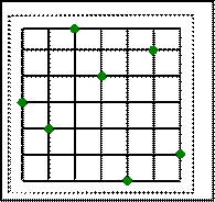
Figure 1: Example linear sensor grid where each horizontal and vertical segment is a road and green dots are the processors.
������������� -*--- --*-- ---*- --*-- --*-- --*--
������������� *-*-* *-*-* *-*-* -*-*- -*-*- -*-*-
������������� -*-*- -*-*- -*-*- *-*-* *-*-* *-*-*
������������� --*-- --*-- --*-- -*--- --*-- ---*-
Figure 2: The six optimal grid placements for 4 rows, 5 columns, and 7 processors on evenly spaced cables without weights.
Table 1: Number of optimal processor configurations and cost of that optimal configuration, for grids with C columns, R, rows, and P processors without weights.
|
|
P=2 |
P=3 |
P=4 |
P=5 |
P=6 |
P=7 |
P=8 |
P=9 |
P= 10 |
P= 11 |
P=12 |
|
C=2, R=2 |
2/ 20 |
4/16 |
1/12 |
|
|
|
|
|
|
|
|
|
C=3, R=2 |
|
2/29 |
8/ 25 |
6/ 21 |
1/17 |
|
|
|
|
|
|
|
C=3, R=3 |
|
6/56 |
1/ 44 |
6/ 40 |
22/ 36 |
24/32 |
9/ 28 |
1/24 |
|
|
|
|
C=4, R=2 |
|
|
2/ 38 |
12/34 |
18/ 30 |
8/ 26 |
1/ 22 |
|
|
|
|
|
C=4, R=3 |
|
|
2/ 73 |
6/ 63 |
2/ 55 |
18/51 |
61/47 |
84/ 43 |
49/39 |
12/ 35 |
1/31 |
|
C=4, R=4 |
|
|
24/120 |
4/ 100 |
2/ 88 |
4/ 80 |
2/ 72 |
20/ 68 |
114/ 64 |
304/ 60 |
405/ 56 |
|
C=5, R=2 |
|
|
|
2/ 47 |
16/ 43 |
38/39 |
32/35 |
10/ 31 |
1/27 |
|
|
|
C=5, R=3 |
|
|
|
4/ 92 |
19/ 82 |
1/ 70 |
9/ 66 |
53/ 62 |
174/ 58 |
276/ 54 |
215/ 50 |
|
C=5, R=4 |
|
|
|
12/ 149 |
2/ 127 |
6/ 117 |
2/ 105 |
4/ 97 |
2/89 |
24/ 85 |
170/ 81 |
|
C=5, R=5 |
|
|
|
120/ 220 |
2/ 188 |
4/ 168 |
33/ 156 |
1/ 140 |
4/132 |
22/ 124 |
1/112 |
����������������������� --*--�� -*-*-��
����������������������� -*-*-�� *-*-*
����������������������� *-*-*�� -*-*-
����������������������� -*-*-�� *-*-*
����������������������� --*--�� -*-*-
Figure 3: The two optimal sensor configurations for 5 columns and 5 rows.
Beyond mirror reflections and rotations, we can also
prove a class of transforms that maintain optimality of configurations.� Theorem:
In a uniform grid with processors assigned to grid intersections, if a
configuration with two processors at ![]() and
and ![]() is reliability-optimal, then replacing
those processors with ones at
is reliability-optimal, then replacing
those processors with ones at ![]() and
and ![]() �is also reliability-optimal, provided no
other processors assigned to within or on the rectangle bounded by the four
locations.� Proof: Since reliability varies with the square of the
lengths of the sensors on either sides of the processor in either dimension,
this sum for the first configuration for
�is also reliability-optimal, provided no
other processors assigned to within or on the rectangle bounded by the four
locations.� Proof: Since reliability varies with the square of the
lengths of the sensors on either sides of the processor in either dimension,
this sum for the first configuration for![]() and
and![]() lines in the first and second dimensions
respectively is:
lines in the first and second dimensions
respectively is:
![]()
and the sum for the second configuration is:
![]()
and the two formulae are identical.
Corollary: A reliability-optimal placement of N processors to an N by N grid of linear sensors is to have them along a diagonal of the array.� Proof:� On N by N grid, each processor must be on a separate row and separate column to cover all of them.� Thus they satisfy the conditions for the above theorem, and can be rearranged along a diagonal.
So far we have assumed the all locations are equally important to monitor.� Otherwise, we can assign weights to indicate importance, either on locations or on rows and columns.� For instance, if we assign weights of [1,2,1,1,1] to the vertical cables and [1,1,2,1] to the horizontal cables in Figure 2, the fourth configuration is the unique optimal solution at a cost of 136.� Weight variety tends to ensure that there is a single unique optimum configuration.
2.3 Bent cables
An alternative to a cable grid is to use a single cable
bent into a configuration giving good coverage of a desired area.� This would
be desirable if the dimensions of the area we want to cover are much less than
the usable cable length C.� The problem of finding optimal paths to cover an area
has been addressed by research on physical search methods7.� Two methods
are the �lawnmower� pattern (Figure 4) and the spiral.� The lawnmower pattern
is good for coverage of rectangular areas, and uses parallel straight segments
at distance 2D in alternating directions connected by orthogonal segments at alternating
ends.� Then to cover a rectangular area of length L and width W we need a cable
of length ![]() .�
If the length is not equal to the width, we save length by running the segments
in the direction of the length rather than the width. �A lawnmower pattern has
been used to effectively monitor vehicles on roads8.
.�
If the length is not equal to the width, we save length by running the segments
in the direction of the length rather than the width. �A lawnmower pattern has
been used to effectively monitor vehicles on roads8.
A spiral is good for coverage of roughly circular areas,
and the type needed here is the Archimedean spiral ![]() �which maintains a constant
distance of 2D to itself as it expands outwards (Figure 5).� Then the necessary
length of the spiral to cover a circle of radius R must subtend an angle of
�which maintains a constant
distance of 2D to itself as it expands outwards (Figure 5).� Then the necessary
length of the spiral to cover a circle of radius R must subtend an angle of ![]() �and its length is:
�and its length is: ![]() .� Figure 5 shows how
the spiral for D=5.5 can be used to cover a circle of radius approximately 16.
.� Figure 5 shows how
the spiral for D=5.5 can be used to cover a circle of radius approximately 16.

Figure 4: "Lawnmower" pattern for deployment of a single cable.
![]()
![]()
![]()
![]()
![]()
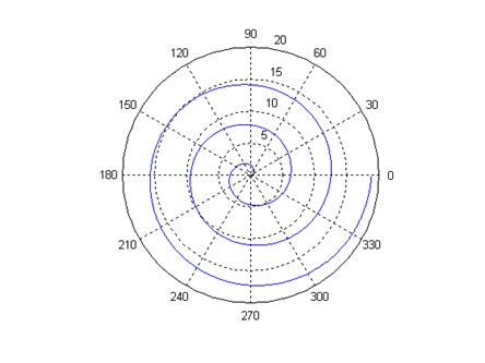
Figure 5: Archimedean spiral.
Spirals are better than lawnmower patterns when they fit
an area.� Theorem: Smoothly curved deployments provide better area
coverage per unit distance along the cable than abruptly turning deployments.� Proof:
Compare two ways of deploying the cable to change its direction, an abrupt right-angle
turn and a smooth arc of 90 degrees of a circle.� A straight cable will provide
sensor coverage of an area of 2D width times the length of the cable.� But at a
right-angle turn, it will cover an area of ![]() �to the outside of the turn while
redundantly covering at area of
�to the outside of the turn while
redundantly covering at area of ![]() �on the inside of the turn, for a net
loss of coverage of
�on the inside of the turn, for a net
loss of coverage of ![]() .�
On a smooth circular arc of 90 degrees and radius R, the area covered to the
outside of the arc is
.�
On a smooth circular arc of 90 degrees and radius R, the area covered to the
outside of the arc is ![]() , and the area covered to the inside of
the arc is
, and the area covered to the inside of
the arc is ![]() .�
So the difference in area covered by the arc with the area covered by a
straight line of the same length is
.�
So the difference in area covered by the arc with the area covered by a
straight line of the same length is ![]() .� Hence the arc is preferable.
.� Hence the arc is preferable.
Note that as the curvature of a curve increases and approaches that of an abrupt turn, the area covered near the turn is covered less and less well.� At some point this coverage may provide too much noise to be adequate.� In addition, fiber-optic cables that bend with more than a certain rate of curvature lose total internal reflection and thus energy into the cable packaging.� Thus there are practical limits to how much a cable should bend.
As for the optimal placement of the processors along an Archimedean
spiral, the curvature of the line does not matter to the reliability analysis,
and they should be evenly spaced along the curve following our discussion of
section 2.1.� A spiral of that subtends angle ![]() �(i.e. covers that bearing angle as it
rotates about the start point through its full length) will have length
�(i.e. covers that bearing angle as it
rotates about the start point through its full length) will have length ![]() �which for large
�which for large ![]() �is approximately
�is approximately ![]() .� Hence for a cable
of length
.� Hence for a cable
of length ![]() ,
M processors should be optimally placed at bearings from the start of the cable
determined for k=1 to M by
,
M processors should be optimally placed at bearings from the start of the cable
determined for k=1 to M by ![]() .� Figure 5 shows these points as dots
for M=5.
.� Figure 5 shows these points as dots
for M=5.
2.4 Deployment over irregular areas
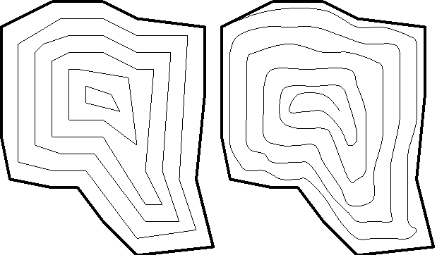
A problem in covering terrain with cable sensors is how
to cover irregular areas.� With cable grids, coverage can be built from
rectangular areas.� An alternative with spirals is to lay them along the length
of the region to be covered (Figure 6).� Two spirals can be placed end to end
for more rectangular coverage.� Large spirals cover an approximately circular
extent, and so a set of spirals placed end to end leave coverage gaps equal to ![]() �of the total area.�
These can be filled with smaller spirals or by grid placements.� Paired spirals
can be duplicated like wallpaper patterns to file arbitrary rectangular areas
whose length to width ratio is a ratio of small integers.
�of the total area.�
These can be filled with smaller spirals or by grid placements.� Paired spirals
can be duplicated like wallpaper patterns to file arbitrary rectangular areas
whose length to width ratio is a ratio of small integers.

|
A key problem for analogous research on search and rescue is how to handle an irregular deployment area.� If we follow a grid approach, we can extend the sensor cables horizontally and vertically at a distance of 2D apart until they reach the edges of an irregular deployment area.� But this may lay unnecessary cables too close to the boundaries.� A more efficient approach is to follow the boundary at progressive integer multiples of 2D from it (the left diagram of Figure 7), much like contour lines in topographic maps.� Each closed loop can be a separate set of cables, or several short curves can be connected by short segments of length 2D as with lawnmower patterns.
|
�����������
�Alternatively, create an irregular spiral by following a line that starts on the boundary and smoothly increases its distance into the deployment area until it is 2D after one circuit, then 4D after two circuits, and so on, as in the right diagram in Figure 7.� Tracing a path that is a distance 2D from another is an interesting problem in computational geometry because it requires more than following the boundary locally.� During tracing, a nonadjacent portion of the boundary may also come within distance 2D because of turns or curves on the boundary.� A simple method, that involves on the average only a small amount of wasted effort, is to trace the closest path or boundary at distance 2D until it intersects some other portion of the boundary; then back up distance D along the trace and erase that portion, then continue tracing while maintaining distance 2D from the new boundary.
2.5 Deployment over terrain not� equicost
We often know that certain parts of the terrain are more
likely to see activity than others.� Or we may know that certain parts of the
terrain are more valuable to monitor.� In either case we can assign a "importance"
function i(x,y) which is a continuous function of the terrain location.� The i
could be a result of convolving a function of coverage quality with offset from
the sensor, ![]() ,
with the probability distribution of targets, t(x,y).� Then the problem can be
turned into a problem of minimizing an "unimportance" cost
,
with the probability distribution of targets, t(x,y).� Then the problem can be
turned into a problem of minimizing an "unimportance" cost ![]() �for a path where I
is the maximum possible importance value.
�for a path where I
is the maximum possible importance value.
This is a classic problem in the calculus of variations
if c is a continuous function with continuous derivatives.� But we cannot
assume that here because there are absolute limits to how far away a signal can
be and still be detected.� An alternative is a heuristic approach based on
solutions to analogous problems in optimal path planning for robots9.�
We can model the terrain as being comprised of polygonal regions with uniform
values of c within each polygon.� Then it can be shown that optimal paths do
not curve and only turn on boundaries between regions.� The turns must obey
Snell's law on the boundaries, which means that ![]() �must be the same on both sides, where q is the angle the path makes with respect to
normal to the boundary (the "angle of incidence").� Thus we can find locally
optimal paths by a ray-tracing approach where we send paths out from a starting
point and obey Snell's Law at each boundary.� For a fixed length of cable, we
can compute the total costs over that length for a range of starting bearings,
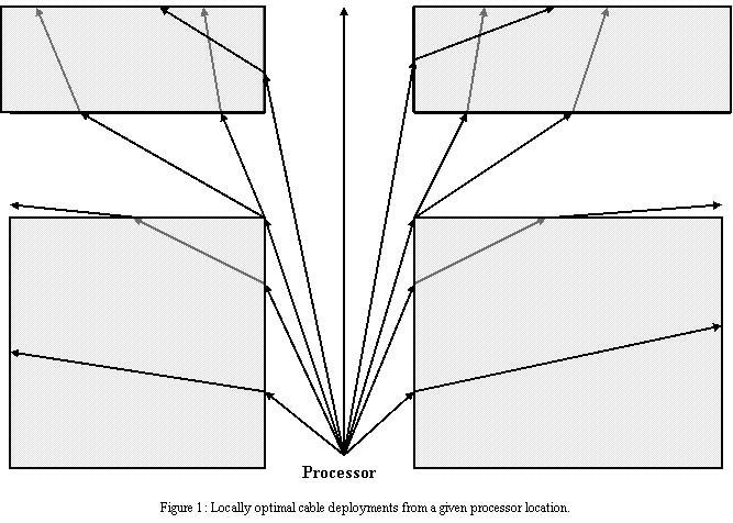
and choose the minimum-cost one as the highest-coverage path.� Figure 8 shows
an example for terrain at a road intersection where the value of covering the
roads (the clear area) is twice that of covering the sides of the roads (the
shaded areas), and a cable is strung from a processor located in the bottom
center.
�must be the same on both sides, where q is the angle the path makes with respect to
normal to the boundary (the "angle of incidence").� Thus we can find locally
optimal paths by a ray-tracing approach where we send paths out from a starting
point and obey Snell's Law at each boundary.� For a fixed length of cable, we
can compute the total costs over that length for a range of starting bearings,
and choose the minimum-cost one as the highest-coverage path.� Figure 8 shows
an example for terrain at a road intersection where the value of covering the
roads (the clear area) is twice that of covering the sides of the roads (the
shaded areas), and a cable is strung from a processor located in the bottom
center.
��������������������������������������������������������������������������������������
3. Tracking with the Cable sensors
Tracking with optic-cable sensors poses interesting problems which have some differences from those of traditional radial-sensitivity sensors.� With most of the proposed technology like (Kirkendall et al, 2007), we will get linear features of generally shallow slopes in a time versus distance plot.� Figure 9 shows a hypothetical time-distance plot with four sources moving in range of a cable laid along a straight line.

Figure 9: Example data from an optic-cable sensor.
3.1 Image analysis
We can use traditional edge-finding techniques from computer vision to find trajectories of people and vehicles in this time-distance image.� If the cable lies along a road or route, normal human activity will appear as straight line segments.� Analysis of an edge will suggest the mass of the tracked object (from intensity), its pattern of distance from the cable (from its intensity variation), its close relationship to other objects moving with it (from closely coincident tracks), and its manner of locomotion or activity (from the evenness along the track).� Intensity should increase out of noise when a track enters the sensor area, and should decrease to noise when a track leaves the sensor area..� So although we cannot measure distance of activity from the cable directly, we have clues as to what is happening.�
Several classes of suspicious behavior can be identified in a time-distance image.� Excavation near the cable is easy to detect as large intermittent signals in a single location with 0.5-10 second periodicity of the peaks.� Abrupt changes in speed and direction will appear as changes in the slope of the track and can be easily noticed; our previous work10 confirmed the importance of recognizing nonzero accelerations for detecting suspicious behavior.� Stopping abruptly will be noted as a discontinuity in a track when its intensity is well above noise.� Some loitering can be detected as unusually slow travel along the axis of the cable; other loitering can be detected as periodic returns to the same locations of the same kind of signal.� It is also important to store statistics over periods of time to learn context for interpreting locations along the cable with special characteristics, such as doors of buildings for people, gathering places like markets for people, and bottlenecks like traffic lights and stop signs for vehicles.
Two kinds of error are possible with signals from the
cable: errors in time of events, and errors in location of events along the
cable.� Both are ultimately due to errors in measurement of times since
location is estimated by reflection time.� But the estimation of the time of
events is more accurate than the estimation of the location from time because the
former measures a process that is several feet per second, whereas the latter
measures a process at the speed of light.� Assume that there is a normally
distributed error in location with standard deviation ![]() .� Then there will be a
normally distributed error in velocity of
.� Then there will be a
normally distributed error in velocity of ![]() �for two points, and a normally
distributed error in acceleration of
�for two points, and a normally
distributed error in acceleration of ![]() �for three points.� Hence the acceleration
error for N points will be
�for three points.� Hence the acceleration
error for N points will be ![]() .� Thus if we encounter a difference in
accelerations between two adjacent nonoverlapping time intervals of D, it will
be significant if it is more than say 3 standard deviations or
.� Thus if we encounter a difference in
accelerations between two adjacent nonoverlapping time intervals of D, it will
be significant if it is more than say 3 standard deviations or ![]() .� This then is our
criterion of potentially suspicious behavior due to acceleration changes along
the cable length.� Inconsistency in the motion of a pedestrian or vehicle can
be considered similarly to the sampling error.� If it is normally distributed,
its variance adds to the sampling variance with
.� This then is our
criterion of potentially suspicious behavior due to acceleration changes along
the cable length.� Inconsistency in the motion of a pedestrian or vehicle can
be considered similarly to the sampling error.� If it is normally distributed,
its variance adds to the sampling variance with ![]() .� Rather than comparing slopes directly,
it is best to compare the fit of new points to the line estimated for previous
points, which allows for using the same formula for finding changes in speed
and direction.
.� Rather than comparing slopes directly,
it is best to compare the fit of new points to the line estimated for previous
points, which allows for using the same formula for finding changes in speed
and direction.
3.2 Localization with bent cables
Motion perpendicular to the cable is more difficult to recognize than motion along the cable.� We can use the square root of the signal strength as a rough measure of distance of activity from the cable, but this will be confounded with noise and variations in the signal strength itself.� Smoothing over time will be essential to address such effects, but smoothing reduces the real effects as well.
Using a bent cable provides some new capabilities in
localization, however.� That is because a subject near a bend towards them in
the cable provides two local maxima before and after the bend.� This has the
effect of localizing them along two intersecting lines.� This effect works with
any bend in the cable, but is easiest to use for localizing if the bend involves
a turn of 90 degrees.� Consider the cable deployment with an indefinitely
repeated pattern of right-angle turns in opposite directions as in Figure 10.� If
D is the maximum sensing distance, we should alternate segments of length D
with segments of length 2D to get complete coverage along an indefinitely long
rectangular area of width D.� Then we will expect to receive two signal maxima
for any subject in the rectangular area.� Calling their distances along the
cable from its end ![]() �and
�and
![]() �with
�with ![]() , and assuming
, and assuming ![]() �where
�where ![]() , we can localize a
subject relative to corner n at �
, we can localize a
subject relative to corner n at �![]() . ��If the cable starts at (0,0) and
extends in the positive x direction, corner n has location
. ��If the cable starts at (0,0) and
extends in the positive x direction, corner n has location ![]() .� This deployment requires
only three times the cable length per unit of coverage area compared to that of
a single straight-line deployment providing only a single distance
measurement.� Note that signal strength can provide confirmation in matching
the signal peaks when there are many, since strengths should vary as the
inverse square of the distance.
.� This deployment requires
only three times the cable length per unit of coverage area compared to that of
a single straight-line deployment providing only a single distance
measurement.� Note that signal strength can provide confirmation in matching
the signal peaks when there are many, since strengths should vary as the
inverse square of the distance.
 |
3.3 Data transmission
Suspicious behavior should be reported as soon as it is detected, preferably to a single data-collection site.� But communication between processors is also necessary to provide the handover of tracks from one processor to another, as when a pedestrian turns from one road onto another.� Explicit handover helps accuracy because the new processor can take advantage of what the old processor has already learned about track.� Also, turns from one road to another are not suspicious, and recognizing them using communications between two processors will reduce the false positive rate on detecting suspicious behavior.� On a road grid with cables along each road, explicit handover between cable processors can be done everytime a subject approaches a known cable intersection.� Handover can be accomplished by sending a message to the processor of the other cable there giving the cable number and the parameters of the subject including average speed in several time windows, speed variance, average signal strength, and signal-strength variance..� If a turn occurs, it can be confirmed by a signal increase on the new cable to a plateau at the time of the turn, simultaneous with a plateau on the old cable followed by a decrease starting at the time of the turn.
Recognition of loitering behavior is aided by coordinated analysis of multiple cables by their processors.� They can look for multiple changes of direction in the path, as well as looping back to previous locations.� This is most easily done at a single collection site that can view all the tracks from all the cables.� But it can also be done more distributively if handovers between cables include all the previous information for a track.
4. Conclusions
Cable sensors offer new capabilities not offered by point sensors since they can provide uniform coverage along a path.� But they also raise new deployment issues that do not arise with point sensors, since wireless communication is less important for cables, reliability is more important, and deployment is more difficult.� It is likely that initial deployments will try too much to duplicate point deployments to their detriment.� Nonetheless, cable sensors are likely here to stay because they provide major advantages in cost-performance tradeoffs for common tasks such as automated monitoring of perimeters and borders.
Acknowledgments
This research was supported by the National Science Foundation under grant 0729696.� The views expressed are those of the author and do not reflect the policy of U.S. Government.
References
[1] Nash, P., "Review of interferometic optical fibre hydrophone technology," IEEE Proc. on Radar Sonar and Navigation, 143, 204-209 (1996).
[2] Kirkendall, C., Bartoloa, R., Salzano, J., and Daley, K., "Distributed fiber optic sensing for homeland security," NRL Review, 195-196 (2007).
[3] Madsen, C., Snider, T., Atkins, R., and Simcik, J., "Real-time processing of a phase-sensitive distributed fiber optic perimeter sensor," Proc. SPIE Vol. 6943, Symposium on Sensors, Command and Control, Communications, and Intelligence, Orlando, FL (2008).
[4] Juarez, J., and Taylor, H., "Distributed fiber optic intrusion sensor system for monitoring long perimeters," Proc. of SPIE Vol. 5778, Sensors and C3I Technologies for Homeland Security and Homeland Defense IV, Bellingham, WA, 692-703 (2005).�
[5] Lang, L.,� "Overview of search theory, part 1," Technical Rescue, 50, 28-31 (2008).
[6] Harres, D., "Built-in test for fiber optic networks enabled by OTDR," Proc. 25th Digital Avionics Systems Conference, Portland, OR, 1-8 (2006).
[7] Champagne, L., Carl, R., and Hill, R., "Agents models II: search theory, agent-based simulation, and U-boats in the Bay of Biscay," Proc. 35th Winter Simulation Conference, New Orleans, LA, 991-998 (2003).
[8] Hill, D., Nash, P., and Sanders, N., "Vehicle weight-in-motion using multiplexed interferometric sensors,", 15th Optical Fiber Sensor Conference Technical Digest, Portland, OR, 1, 383-386 (2002).
[9] Rowe, N., and Alexander, R., "Finding optimal-path maps for path planning across weighted regions," �International Journal of Robotics Research, 19(2), 83-95 (2000).
[10] Rowe, N., "Interpreting coordinated and suspicious behavior in a sensor field," Proc. of the Meeting of the Military Sensing Symposium Specialty Group on Battlespace Acoustic and Seismic Sensing, Magnetic and Electric Field Sensors, Laurel, MD (2008).