An Efficient Snell's-Law Method for Optimal-Path Planning Across Multiple Two-dimensional Irregular Homogeneous-Cost Regions
Neil C. Rowe and R. F. Richbourg
Department of Computer Science
Code 52Rp, U.S. Naval Postgraduate School Monterey, CA 93943 USA
Abstract
We are exploring a new approach to high-level
optimal-path planning when homogeneous irregularly-shaped regions of a plane
have different traversal costs per unit distance. It is based on the simple
idea that optimal paths must be straight in homogeneous regions, and so those
regions need not be subdivided for path planning. Our approach uses optics
analogies, ray tracing, and Snell's Law, and reduces the problem to an
efficient graph search with a variety of pruning criteria. The time and space of
our algorithm is ![]() in
an intuitively average case, where V is the number of region vertices. In
experiments in which space is held constant, an implementation of our algorithm
was not only dramatically faster but gave better-cost solution paths than a
representative implementation of the chief competing technique, grid-based
wavefront propagation. This appears due to the quite different and considerably
smaller search space required for our more intelligent algorithm.
in
an intuitively average case, where V is the number of region vertices. In
experiments in which space is held constant, an implementation of our algorithm
was not only dramatically faster but gave better-cost solution paths than a
representative implementation of the chief competing technique, grid-based
wavefront propagation. This appears due to the quite different and considerably
smaller search space required for our more intelligent algorithm.
|This work was supported in part by the U. S. Army Combat Developments Experimentation Center under MIPR ATEC 88-86. R. F. Richbourg is currently with the Office of Artificial Intelligence Analysis and Evaluation, U.S. Military Academy, West Point, New York, USA. This paper appeared in International Journal of Robotics Research, 9, no. 6 (December 1990), 48-66. The equations were redrawn in 2008.
Introduction
We address here the problem of optimal-path planning for autonomous mobile agents in two dimensions. In particular, we are concerned with large-scale or "high-level" path planning in which the start and goal points are specified, and the size and dimensions of the agent are negligible in comparison to the geometry of the path. And consistent with the term "large-scale", we assume reasonably complete knowledge of the features of the two-dimensional space across which we are planning, including not only the locations and dimensions of obstacles for traversal, but traversal costs per unit distance for homogeneous regions within the two-dimension space or "terrain". The primary intended application of our work is off-road navigation by autonomous vehicles, but it also applies to planning military operations and constructing permanent linear features such as pipelines.
In defense of our concern for optimality of proposed paths, we argue that minimizing a cost is natural and desirable in most path-planning problems, be it an energy expenditure, traversal time, total probability of accident, or some weighted sum of the three. We will show that the cost of finding an optimal path by our algorithm is not unreasonable, making finding nonoptimal paths often pointless. In defense of our assumption of reasonably detailed terrain-cost information, standard terrain maps and aerial surveying such as that done by the United States Defense Mapping Agency already provide detailed information for most of the earth's surface for planning at a resolution of 100 meters. The surface geometry, composition, and vegetation information provided from such sources are used in the calculations of the Army Mobility Model (AMM) (Rula and Nuttall 1971; Turnage and Smith 1983) to assign cost-per-unit-traversal-distance (infinite for obstacles) for homogeneous areas of the terrain, not necessarily regular, for various kinds of vehicles, with especial emphasis on wheeled vehicles. Our work is predicated on this AMM model and the databases used by it, since they are quite general and cover most overland robotic vehicles proposed, not just military vehicles. We do not have the space here to explain in detail the assumptions used in the AMM, the result of two decades of analysis and experimentation. The model is isotropic, or assumes that traversal direction does not affect cost (other recent work of ours (Rowe and Ross 1988) has addressed this oversimplification). We have experimented with the AMM model on terrain information at a resolution of 12.5 meters, typical of high-priority military terrain, so this will be our formal definition of "large-scale path planning"; even at that resolution, agent size has little import.
The chief innovation of our work is its ability to reason about irregular terrain regions of arbitrary size and shape in path planning, which are possible output from the AMM model. With an irregular-shape representation, terrain features can be better modeled than with the uniform grid that is used in nearly all other approaches to this problem. But such a representation requires a more complex algorithm to reason about what happens to paths on boundaries of regions. Our approach sees an exact analogy between this problem and the paths of light rays in optical media, whose paths obey Fermat's principle. While some theoretical groundwork has been previously published for this approach (Richbourg et al 1987; Rowe 1989; Mitchell 1988) we believe we are the first to implement it.
Previous work
Wavefront-propagation methods
The standard algorithm for finding optimal paths on terrain with a known cost map is a dynamic-programming "wavefront propagation" (Chavez and Meystel 1984; Graglia and Meystel 1987; Parodi 1985; Witkowski 1983; Mitchell et al 1987). (Note that path-finding methods that search a visibility graph of region vertices (Lozano-Perez and Wesley 1979) apply to terrain with only obstacles, not regions of varying cost; and methods that designate "good" areas of free space (Brooks 1983; Crowley 1984; Rueb and Wong 1987) do not give optimal paths.) Terrain is modeled by a uniform "grid" or tessellation of cells of uniform size and shape. Each cell has an associated cost which represents an average cost-per-unit-traversal-distance for the terrain within the cell. The algorithm works by expanding a wavefront (initially approximately circular) about the start point, much in the way that a stone dropped in a smooth pool of water creates ever-expanding ringlets of disturbance in the surface of the water. In the algorithm, the wavefront is expanded at varying rates along its circumference in a way proportional to the reciprocal of the traversal costs for the underlying cells, so the wavefront moves more slowly through high-cost cells. The algorithm stops when the goal point is encountered, and back pointers are used to recover the path that was taken from the start point to that goal point as the wavefront expanded.
Wavefront-propagation algorithms have many variants. But all versions can have certain problems. These problems do not always matter, and there are many applications, such as terrain with a uniformly high level of variation in traversal characteristics, or situations needing simple software, for which wavefront propagation is appropriate and preferable to anything else. But wavefront propagation is not good for all path planning.
First, the imposition of a fixed grid on terrain is arbitrary and is not likely to reflect the organization of the real terrain, causing problems when widely different terrain is averaged within a cell. Figure 1 provides an example: if the original 4 by 6 array of cost values needs to be compressed into eight words of data, the averaging necessary for a regular grid clearly gives a poorer representation of the terrain than the irregular representation with a triangular region embedded inside a background region, whose vertices can be described with six numbers. For real-world paths we will need real terrain databases, which usually store data in the form of regular arrays; but we are interested here only in high-level path planning for which at least some aggregation of that raw data must be performed to enable reasonably quick answers.
Figure 1
Second, it is hard to pick the right grid size, because the level of detail necessary in some portions of the map for good path planning there may be quite different than the level of detail needed elsewhere; an irregular terrain representation can take this in stride. Figure 2 gives an example map, where a uniform grid must either sacrifice fine detail of the upper right corner or wastefully create many identical cells in the rest of the terrain. But algorithms for nonuniform grids are considerably more complicated.
Figure 2
Third, the method is predisposed towards propagation in certain directions; for instance, on a square grid, horizontal, vertical, and diagonal directions of traversal are unfairly preferred with most implementations. But there are some tricks to reduce this problem, discussed in the next section.
Fourth, wavefront-propagation algorithms waste computation, since they blindly explore everywhere. While some simple tricks can rule out certain directions of advance, the uninformed nature of the search process in wavefront propagation can give behavior that appears foolish.
Fifth, wavefront propagation on multi-cost terrain can have difficulties with arithmetic roundoff errors. If a region has a uniform traversal cost, the error in approximation will be multiplied by the length of the path in cells. While large uniform regions are statistically unlikely in uneven terrain, they can arise with manmade terrain.
Sixth, although this is rarely recognized, wavefront-propagation algorithms are incapable even in principle of obtaining optimal solutions in the limit when the number of grid cells modeling some fixed terrain area approaches infinity, because of the "digital bias" effect (Mitchell et al 1987), that solution paths not following the "natural" directions of the grid tend to be longer than necessary because of the "zigzagging". To illustrate, consider a starting point inside a forest and a goal point in a field adjacent the forest. See the top diagram in Figure 3; suppose the forest region is on the left and the field on the right, and the starting point in the lower left corner of the upper box, and the goal point in the upper right corner. Assume the forest and the field are reasonably homogeneous in this vicinity. Suppose (as often with cultivated fields) that the boundary between the two areas is abrupt, and suppose this boundary is a straight line running 14 degrees west of north. Assume the cost of traversing the forest per unit distance is 7 units, and the field 2. Then the optimal path, as verified by the methods described later in this paper, is shown in the upper box. The middle box shows the solution for a four-neighbor wavefront propagation on a 13 by 12 grid, and the lower box on a 26 by 24 grid. (Eight-neighbor propagation programs are more common, and analogous inaccuracies occur, but their illustration would be less dramatic.) Both wavefront propagations give jagged paths due to the permissible directions of propagation, paths which are hardly reasonable for an agent to follow exactly, unlike the path in the top box. Furthermore, the cost of the paths found by the three methods are 17.2, 22.6, and 22.1 respectively, so both wavefront-propagation methods are significantly worse than the true optimal path in cost. While the high-resolution wavefront propagation was a little better, that mostly reflected a lucky coincidence in its problem representation, and is not generally true; in fact, high-resolution wavefront-propagation searches can give significantly worse results than low-resolution searches (though both errors can be bounded). At any rate, the use of all those vertical and horizontal segments virtually guarantees that the solution paths found by basic wavefront-propagation algorithms will be significantly worse than the true optimal solution.
Figure 3
Note that all the above objections to wavefront propagation are far more serious, except the third and fourth which are equally serious, for multi-cost terrain than for terrain with only obstacles. Thus the simplicity and popularity of propagation on obstacle-only single-index terrain should not blind us to the serious additional difficulties of extending it to multiple terrain costs; weighting of cells introduces many serious implementation problems. But multiple terrain costs are essential to accurately modeling nearly any outdoor terrain.
Improved wavefront propagation
Various fixes have been proposed to the basic wavefront-propagation algorithm to address these problems, especially the non-optimality in the solutions generated. Certainly it helps to use the A* search algorithm rather than branch-and-bound at a local level (Graglia and Meystel 1987; Mitchell et al 1987), but the time improvement was rather small in a variety of experiments we conducted (Richbourg, 1987). (Note that use of A* does not affect the propagation-direction problem, as the bias arises from inaccurate cost calculation along a path, not in estimating its future potential.) A more significant variant (Graglia and Meystel 1987; Mitchell et al 1987) is to allow more complex forms of connectivity between the cells to enable a larger number of possible directions of traversal at the local level. But all these other forms of connectivity require an effectively lower resolution in the terrain representation. For instance, to get 16 possible traversal angles, we must skip cells in some directions we travel, meaning the grid must be twice as long and wide (four times as big) to represent terrain features adequately as with basic eight-neighbor propagation. Furthermore, this approach does not eliminate path jaggedness or non-optimality, just reduces it by increasing the number of preferred directions.
A second way to improve paths is to do repeated propagations on successively more detailed representations of the terrain, using results of earlier searches to guide paths for later searches (Graglia and Meystel 1987; Kambhampati and Davis 1986; Metea and Tsai 1987). But optimality guarantees are virtually impossible with even two levels of hierarchy; for instance, Figure 4 shows a situation where the solution to a four-neighbor search on a 6 by 6 terrain representation is the extreme opposite of the solution to a search on a 3 by 3 representation obtained from the first by cell summation. In the top picture, the optimal path follows clockwise along the region boundary from the Start to the Goal and costs 220, and the path following counterclockwise along the boundary costs 231; whereas in the lower picture, the corresponding costs are 206 and 190, and the counterclockwise path is optimal. (Those totals count half of the cost for the start and goal cells.) In general, it is impossible to predict when a terrain will give markedly differently optimal paths at one level of detail than another, and thus hierarchical reasoning cannot be trusted when optimality is desired.
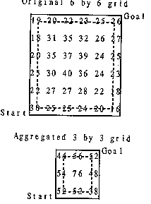
Figure 4
Finally, a third way to improve the paths produced by wavefront-propagation methods is to "straighten" them, either by shortcutting sharp turns (Mitchell et al 1987), fitting straight lines to portions of the path generated (Mitchell et al 1987), or iterative smoothing (Thorpe 1984). But again this does not guarantee an optimal path. For one thing, if the truncation of the path within a homogeneous-cost region does not include an exact multiple of the number of "cycles" of the zigzagging composing the path, the best-fit line will be askew. This skewness can be significant in paths crossing many regions. A more fundamental objection can be raised to the straightening process, however: since optimal paths within homogeneous isotropic regions are always straight, why represent such regions with multiple cells and add unnecessary computation? Wouldn't it make more sense to reason about a large region as a whole, despite possible boundary irregularity? Then none of the ugly tricks just discussed would be necessary.
Previous work: the Continuous Dijkstra Algorithm (CDA)
Independent of our own preliminary work (Richbourg et al 1987), Mitchell (Mitchell 1988; Mitchell and Papadimitriou 1990) developed developed the "Continuous Dijkstra Algorithm" for this problem. This approach has some similar ideas to the one we will describe. However, the CDA was not designed for practicality but to prove a point: that a certain class of path-planning problems can be solved by an algorithm that is, in the worst case, polynomial in time and space with respect to the number of region-boundary line segments. To achieve this, the algorithm requires the start and goal to be on region boundaries, the regions themselves to be triangular, and imposes certain other restrictions.
We believe that polynomial worst-case bounds are unnecessary for an optimal path-planning algorithm, just as polynomial algorithms for linear programming are unnecessary compared to the Simplex algorithm despite the latter's exponential worst-case performance. We have therefore developed an optimal-path-planning algorithm which, like Simplex, works well on the average. It is robust, efficient, and capable of exploiting many powerful pruning heuristics; though its time and space needs with respect to the number of region-boundary edges in the worst case has not been proven better than exponential, in the average case we can prove them quadratic.
Our algorithm
So we will assume terrain consisting of homogeneous regions, each of a characteristic "index" or cost per unit of traversal distance; for instance, forests can have a high index, fields a low index, and steep cliffs an infinite index. We will further assume, consistent with the practice of surveyors, that region boundaries are polygonal. (Any boundary can be approximated to any arbitrary closeness by some polygon.) For such a terrain model, we can prove that optimal-path planning reduces to a finite search even without imposing a cellular grid. Furthermore, since there is a simple lower bound on completion cost in this search, the A* search algorithm is strongly suggested, among the standard search algorithms of artificial intelligence (Rowe 1988). (Do not confuse this use of A* with its occasional use in wavefront propagation: the search spaces are quite different.)
Snell's Law
Fermat's Principle of optics says that light rays always follow a path
between two locations that is a minimum, maximum, or stationary point (though
usually a minimum) with respect to time. So we can solve path-planning problems
by interpreting terrain as optical media, with the cost per unit traversal
distance ("cost index") analogous to the reciprocal of the speed of
light in the region. We can then "trace rays", determine where an
analogous light ray could go, and rule out the occasional maximal-time and
stationary-point-time paths. Fermat's Principle at a boundary between two
homogeneous regions of different index implies Snell's Law, which explains the
refraction or turning of light rays: ![]() . This gives the angle
. This gives the angle ![]() between the normal to
the region boundary and the light path in region 2, when the path angle from
the normal in (incoming) region 1 is
between the normal to
the region boundary and the light path in region 2, when the path angle from
the normal in (incoming) region 1 is ![]() and the characteristic indices
(cost per unit distance) for the two regions are
and the characteristic indices
(cost per unit distance) for the two regions are ![]() and
and ![]() . This applies equally to light rays and
traversal paths. In essence it describes a necessary local condition that must
hold when any minimum-cost path crosses a boundary between regions of different
traversal characteristics.
. This applies equally to light rays and
traversal paths. In essence it describes a necessary local condition that must
hold when any minimum-cost path crosses a boundary between regions of different
traversal characteristics.
Such analysis is greatly simplified when boundaries are straight, so it is desirable to have polygonal terrain regions; this is straightforward to satisfy in the collection of terrain data, as in specified policy for obtaining data for the Army Mobility Model, or by polygonal fitting to data for evenly-spaced terrain points using standard algorithms of computational geometry. Notice that Snell's Law implies that paths only turn where the cost index changes, so on terrain consisting entirely of homogeneous-cost-index regions, any locally-optimal path between two points must be piecewise-linear.
Well-behaved path subspaces (WBPSs)
Our key to finding the optimal path from a start point S to a goal point G is the finding of "well-behaved path subspaces" (WBPSs). A WBPS from point S is a partition of the set of all locally-optimal paths departing from S such that its paths cross the same region-boundary line segments in the same order, obeying Snell's Law at region boundaries. By "locally-optimal" path we mean any slight path perturbation has higher cost. Figure 5 shows some sample paths within a WBPS; for a certain range of starting headings, all locally-optimal paths from the starting point will cross the four near-horizontal region boundaries in sequence. WBPSs cannot enclose region vertices; for path subspaces that do, we will use the more general term "wedge".
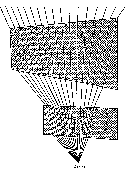
Figure 5
WBPSs are important because they are the terminal nodes for a search tree of wedges, using "search tree" in its conventional artificial-intelligence sense. Consider a subspace of paths that cross the same sequence of cost-region boundaries after starting from some point S, and then head straight to the goal point after crossing the last boundary. We prove in the Appendix that total path cost to the goal is a convex function over the set of all such paths, and hence there is at most one path in a WBPS that is a local cost minimum to the goal. Thus within a WBPS there is at most one locally optimal path from a start to a goal. It can be found by a simple bisection iteration. (Iteration is necessary because there is no closed-form solution for the inverse of the ray tracing problem, of finding a path to a given point.) Then the globally-optimal path from a start to a goal is the best of local optima when all possible paths are apportioned into WBPSs.
A systematic search can provide the WBPSs rooted at a start point S. Since they represent sets of locally-optimal paths crossing the same region boundaries, the two WBPS borders (for instance, the leftmost and rightmost rays in Figure 5) are always locally-optimal paths that each pass through at least one region vertex (for instance, the left upper vertex for the left ray in Figure 5, and the right upper vertex for the right ray). So we can find WBPSs by finding their borders first, by finding the Snell's-Law-obeying paths from the start point S to every region-boundary vertex, in order of increasing distance from S. WBPS finding is a classical search process where wedges are the "agenda" items from which a selection of what to work on next is made, unlike cells which are the agenda items in wavefront propagation. "Branching" means finding a path to a region-boundary point within a wedge and splitting the wedge in two; heuristics can prune wedges from further consideration.
Generally speaking, the idea is to "grow" wedges toward the goal point rather than splitting wedges at random. This is ensured by the distance-to-goal lower-bound cost used in the A* algorithm. Note also that the start and goal points can be reversed and the problem might be easier to solve. But bidirectional simultaneous search is not a good idea because the forward wedges are different from the backward wedges.
Details
That is the basic idea of our algorithm, but there are four important details. First, whenever an optimal path to a vertex V is found, often another "middle" wedge can be created besides the "left" and "right" wedges, one representing paths that follow the single globally-optimal path to V and then diverge. Consider Figure 6, where the shaded region is a higher index than its surroundings, and the black region is an obstacle. Assume locally-optimal paths from the start point S that miss V slightly to the left are bent by refraction 30 degrees left, and paths that miss V slightly to the right are bent 30 degrees right. It seems there is an abrupt change in behavior of optimal paths around point V. This is not so because there is an intermediate class of optimal paths passing through V and turning less than thirty degrees in either direction. To find the optimal path to the goal in this "middle" wedge, we can recursively consider a search problem in which V is the starting point, but with certain initial path-direction restrictions. Points like V are analogous to pinholes in diffraction optics, in being new points of radiation. Middle wedges can also occur with obstacles, as at point U in Figure 6, where a class of paths from S passes through U and then bends around to the "hidden" side of the obstacle. Such obstacle-related middle wedges explain following the exteriors of obstacle boundaries.
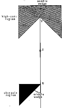
Figure 6
Another detail concerns situations in which Snell's Law (see section 3.1)
claims that the sine of the outgoing angle at a region boundary is greater than
1 (that is, ![]() .
This happens to "grazing" paths, those not sufficiently perpendicular
to the boundary, trying to enter a lower-cost region; for instance in Figure 7,
paths just to the right of the path from S to A to B that is refracted
perpendicular to edge at B. This corresponds to total internal reflection in
optics; in path planning it means that no optimal path crosses the boundary
there. However, there may be a non-reflecting subwedge like that shown that can
cross the region boundary when a bigger wedge cannot. The subwedge is usually
easy to determine because one of its boundaries must hit the region boundary at
the "critical" angle, the arcsine of the ratio of the region indices;
no iterative search for that wedge boundary is needed, unlike forward ray
tracing with Snell's Law.
.
This happens to "grazing" paths, those not sufficiently perpendicular
to the boundary, trying to enter a lower-cost region; for instance in Figure 7,
paths just to the right of the path from S to A to B that is refracted
perpendicular to edge at B. This corresponds to total internal reflection in
optics; in path planning it means that no optimal path crosses the boundary
there. However, there may be a non-reflecting subwedge like that shown that can
cross the region boundary when a bigger wedge cannot. The subwedge is usually
easy to determine because one of its boundaries must hit the region boundary at
the "critical" angle, the arcsine of the ratio of the region indices;
no iterative search for that wedge boundary is needed, unlike forward ray
tracing with Snell's Law.
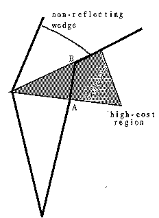
Figure 7
A third detail concerns finding such reflection paths working backwards. Whenever a path runs along a region boundary (the path is then assumed just inside the lower-cost region), a set of locally-optimal paths cut away at the critical angle along it. This set can be reasoned about as another wedge. However, most such wedges will be eliminated quickly by the methods of section 4, so we always in effect give them a large cost surcharge when placing them on the A* agenda.
Fourth, A* search needs a lower bound on the cost through a wedge to the goal, to rate wedges for its agenda. This can be the sum of two lower bounds, one on the cost in the wedge from the start to the farthest-forward boundary known crossed by the wedge, and one on the cost from there to the goal. The first can be proved to occur for the wedge path perpendicular to the last boundary; the second is the lowest possible index times the distance to the goal from the nearest point on the last boundary segment.
The main flowchart of our algorithm is shown in Figure 8. (Richbourg, 1987) gives further details.

Figure 8
An example
Figures 9 and 10 illustrate our computer implementation of our algorithm for a simple example. Figure 9 (the bit map of a display for our actual running program) shows some terrain classified into regions of two kinds; the triangular shaded areas are regions of twice the index (cost per unit distance) of the unshaded areas, and there are no obstacles. The big rectangle represents a "bounding box" within which the solution must lie (see discussion of PM5 in the next section). S marks the start, G the goal. The other points labeled with small letters are used to define all the WBPSs (well-behaved path subspaces) created for this problem. The optimal path found was S to f to n to o to G, at a cost of 7.97; the complete path S to h to r to G was also found, but it costs 9.29. Note point o is a critical-angle cutaway, discussed in the last section.
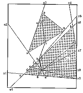
Figure 9
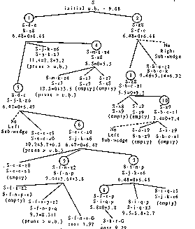
Figure 10
Figure 10 shows the complete A* search tree created by the algorithm for this problem. Each node represents a threefold wedge partition about a vertex. The numbers in the circles give the order in which partitions were made; with partition 9 the optimal solution was found. (Because critical-angle-cutaway wedges have in effect a high surcharge not shown, partition 9 was only made after all non-cutaway wedges were eliminated from the agenda.) For each wedge in the tree, its left and right boundaries are given, as sequences of turn points. Below is either (1) the word "empty", indicating a wedge not containing cost-region vertices, hence ignorable; (2) "prune > u.b.", indicating a wedge pruned because its cost is greater than the global upper bound (see discussion of PM4 in the next section); or (3) the agenda rating, a lower bound on the cost of a path from the S to G that passes through that wedge. The last is shown as the sum of two lower bounds, as explained at the end of the last section, except for the two complete S to G paths. (Nodes 1 and 2 of the tree may be confusing since each represents an entire half plane of rays departing from S; node 1 is rays departing up from the path z8-S-d-c, node 2 those departing down.)
Pruning methods
One consequence of our higher-level representation of the world as meaningfully-shaped regions of homogeneous index is that our algorithm can be more knowledge-based than wavefront-propagation methods for the same path-planning problems. That is, pruning criteria and heuristics can be more easily developed, since they can reference the many possible higher-level features. We now present some major categories of pruning methods. (Our program currently uses all but PM6, PM7, PM8, and PM11, which we decided after analysis would not be cost-effective for the test terrain we were to use.)
PM1: Obstacles. Any wedge whose sides reach the same obstacle-boundary line segment can be pruned whenever the wedge does not enclose the goal or any region-boundary vertices.
PM2: Reflections. Any wedge whose sides reach a boundary line segment for which internal reflection in the same direction occurs for both sides can be pruned, provided the wedge does not enclose the goal or any region-boundary vertices.
PM3: Closed wedges. Any wedge whose sides meet can be pruned, provided it does not enclose the goal or any region-boundary vertices.
PM4: Pruning with a cost upper bound in A* search. Suppose we have an upper bound U on the cost from the start to the goal. The cost of the straight line between them will do if it does not intersect obstacles; if it does, an algorithm like (Lozano-Perez and Wesley 1979) can find the shortest obstacle-avoiding path to use instead. Then any wedge on the agenda rated more than U can be pruned. U can be improved anytime a better path to the goal is found, allowing possibly immediate further agenda pruning.
PM5: Global ellipse limiting. Pruning method PM4 can also be used
preemptively. Given an upper bound U on the cost of the optimal path from start
to goal, D the straight-line distance, and ![]() the lowest cost index possible.
Then the globally-optimal path is contained in an ellipse whose foci are the
start and goal, whose major axis is
the lowest cost index possible.
Then the globally-optimal path is contained in an ellipse whose foci are the
start and goal, whose major axis is ![]() , and whose minor axis is
, and whose minor axis is ![]() . (This follows from
the definition of an ellipse as the locus of points the sum of whose distances
from the foci is constant.) Figure 11 shows an example where the shaded regions
have a cost index 1.77 times the unshaded area; then the straight-line path
between start S and goal G is 45% in high-cost area, at an average cost 1.35
times the optimum, and the bounding ellipse is as shown. So any wedge that does
not enclose a region-boundary vertex within the ellipse can be pruned. But to
save time in our program we use the rectangle ("bounding box")
circumscribing the ellipse; only a little extra area is included.
. (This follows from
the definition of an ellipse as the locus of points the sum of whose distances
from the foci is constant.) Figure 11 shows an example where the shaded regions
have a cost index 1.77 times the unshaded area; then the straight-line path
between start S and goal G is 45% in high-cost area, at an average cost 1.35
times the optimum, and the bounding ellipse is as shown. So any wedge that does
not enclose a region-boundary vertex within the ellipse can be pruned. But to
save time in our program we use the rectangle ("bounding box")
circumscribing the ellipse; only a little extra area is included.
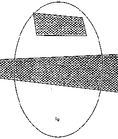
Figure 11
PM6: Cost bounds from dual-graph analysis. After an ellipse has been drawn, we can analyze the regions enclosed to obtain better cost bounds on paths. A dual graph can be constructed where nodes represent regions or region portions, and edges represent region adjacencies. Cost bounds can be computed for every sequence of three connected nodes in this graph, bounds on the cost that can be incurred in the middle node when traveling from the first to the third. They can be determined from the minimum width and maximum length (or necessarily in some cases, the circumference) of the region portions. For instance in Figure 11, if the straight path between S and G is one unit long, the optimal path from S to G must spend a minimum of 0.20 units of distance in the long rectangular high-cost region, a minimum of 0.01 units in the upper high-cost region, a maximum of 0.31 in the lower, and a maximum of 0.37 in the upper; so if the high-cost regions have an index 1.77 times their surroundings, the cost expended in them on the optimal path must be between .37 and 1.20. In general, numbers can be summed for all possible paths between start and goal to get upper and lower bounds on the cost of the optimal path.
PM7: Iterative ellipse improvement. Once an ellipse has been constructed, its interior can be examined, for instance with PM6, to possibly get a better (smaller) upper bound on cost. This implies a narrower ellipse with perhaps an even better upper bound, and so on iteratively.
PM8: Virtual obstacles. Suppose convex region R has index |n sub r|,
and suppose R is bordered by regions of index lower than |n sub s|. Then no
optimal path can enter R except to reach a goal point inside (that is, R is a
"virtual obstacle") if for any pair of points P and Q on the border
of R, the ratio of the shortest distance along the perimeter of R from P to Q
to the straight-line distance between them is less than ![]() .
.
PM9: Corner cutting. Suppose a wedge cuts across a corner of a region of higher index than its surroundings; that is, the wedge crosses two successive boundary line segments of the region, segments meeting at a vertex. Then the wedge can be pruned if the sine of half the angle between the segments is more than the ratio of the indices. This follows because the greatest advantage of a shortcut occurs when it forms an isosceles triangle with the corner vertex.
PM10: Using cached costs of optimal paths. Suppose we want the cost
of the optimal path between points R and S, and we know the cost c(A,B) of the
optimal path between nearby points A and B. Let d(R,A) be the distance of R
from A, d(S,B) the distance of S from B, and ![]() the highest index in the area of
interest. Then an upper bound on the cost from R to S is
the highest index in the area of
interest. Then an upper bound on the cost from R to S is ![]() and a lower bound is
and a lower bound is ![]() . The closer R to A
and S to B, the tighter these bounds. For instance in Figure 12, suppose the
optimal path from C to D is the one-bend path shown; then the optimal path from
A to B is a subpath of the path from C to D; and an upper bound on the cost of
the optimal path from S to G is the cost from S to A plus the cost from G to B
plus the cost of the optimal path from A to B. To facilitate good bounds, we
could prestore optimal costs between evenly-spaced points, or between region
vertices since our algorithm focuses on them. Or we could cache the results of
previous path planning, to provide a simple form of learning from experience.
The more cached costs, the better the search pruning, and the faster the
solution. (We can also cache costs of nonoptimal paths, but they only provide
upper bounds.)
. The closer R to A
and S to B, the tighter these bounds. For instance in Figure 12, suppose the
optimal path from C to D is the one-bend path shown; then the optimal path from
A to B is a subpath of the path from C to D; and an upper bound on the cost of
the optimal path from S to G is the cost from S to A plus the cost from G to B
plus the cost of the optimal path from A to B. To facilitate good bounds, we
could prestore optimal costs between evenly-spaced points, or between region
vertices since our algorithm focuses on them. Or we could cache the results of
previous path planning, to provide a simple form of learning from experience.
The more cached costs, the better the search pruning, and the faster the
solution. (We can also cache costs of nonoptimal paths, but they only provide
upper bounds.)
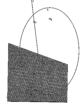
Figure 12
PM11: Using cached optimal paths. No optimal path can intersect another optimal path more than once. (Otherwise there would be two equally-good paths between the two points of intersection.) So any previously-computed optimal path from A to B lying to one side of start S and goal G forms a barrier which the optimal path from S to G cannot cross. If A and B both lie outside the limiting ellipse, and the optimal path between them intersects the ellipse, then the barrier rules out an entire part of the ellipse. For instance in Figure 12, if the C to D path is optimal, it rules out the area to its right side within the ellipse for the optimal path from S to G. This suggests we should store optimal paths between a variety of widely-spaced points.
Performance analysis
Worst-case theoretical analysis
Within the initial ellipse for some problem, let v be the number of region vertices, and let e be the number of region edges. Since all regions are polygons, the number of edges is close to the number of vertices. Regions can share edges and vertices, in which case the number vertices is decreased by one for every shared edge. But even so, O(e) = O(v).
The main loop of the program takes the lowest cost wedge from the agenda, determines the closest search point (a region vertex or the goal) within that wedge, if any, and replaces the wedge on the agenda by up to four subwedges (the left, the middle, the right, and possibly an internal-reflection wedge). Since each wedge partition removes one wedge from the agenda and adds up to four, an upper bound on the total number of wedges created by the algorithm is 3P-2, P the number of partitionings made.
But the number of partitions is not just the number of search points,
because wedges can overlap, and the same search point can be encountered in
more than one wedge. Wedges can be characterized by a permutation of a subset
of all the possible edges and vertices up to the point at which the edge is
explored. An upper bound on the number of such permutations is O(v+e+1)! =
O(v!), where the 1 represents the goal. In the worst case, wedge partition
requires comparing each vertex to the wedge to determine if it is inside, which
requires ![]() time.
So an upper bound on the time complexity of the algorithm is
time.
So an upper bound on the time complexity of the algorithm is ![]() .
.
As for the space complexity, the problem representation requires O(v). But this is negligible compared to the dynamic requirements for the agenda of wedges, which can contain at worst O(v!) wedges. Each wedge description requires one or two vertices for each edge or vertex encountered, which is O(v) in the worst case, so the total space requirements in the worst case are O(v!v).
Figure 13 shows the kind of situation that approaches the worst-case bound. The three high-cost regions between the start and goal can act like optical lenses, "focusing" paths into a narrow band to either side of the straight line connecting start and goal, if costs and dimensions fall within a certain narrow range. Then many wedges at the start point can include the goal point. But such circumstances require exceptional coincidences in the real world.
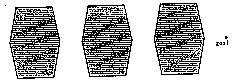
Figure 13
Average-case theoretical analysis
But average-case performance of our algorithm is much better, ![]() . To see this, we will
define "average case" to mean terrain with a statistically even
distribution of features. And as v increases, we will assume that a larger
bounding box is taken on the same terrain, not more regions added to the same
box. We want to know how complexity increases then.
. To see this, we will
define "average case" to mean terrain with a statistically even
distribution of features. And as v increases, we will assume that a larger
bounding box is taken on the same terrain, not more regions added to the same
box. We want to know how complexity increases then.
First observe that refining a wedge selected from the agenda requires examining O(v) vertices, comparing them to the boundaries of the wedge, for which it is almost always sufficient to compare to the two lines representing the indefinite extension of first unexplored part of the wedge. We may in many cases be able to improve on O(v) if we sort region vertices into bins of a two-dimensional grid, or by closeness to some point of interest; the sorting can be done in linear time if we can copy the items to a sparse auxiliary array.
Once the nearest unsolved vertex V for the wedge has been found, an iterative search must find the Snell's-law path in the wedge to V. The time for this fluctuates randomly, but is roughly proportional to the number of edges crossed since a Snell's law calculation must be done at each edge, so the time is O(e) = O(v).
Now if all search points encountered by the algorithm are encountered no
more than once, an upper bound on the number of wedge partitions is |v|, and
thus the average-case performance of the algorithm is ![]() . This result holds for terrain
with few vertices or vertices spaced widely apart.
. This result holds for terrain
with few vertices or vertices spaced widely apart.
Otherwise, there are two kinds of multiple encounter of search points. One kind is the immediate encounter caused by a "focusing vertex" as in Figure 13. The partition of a wedge about such a point can create not only a middle wedge, but the left and right wedges that can intersect both the middle wedge and each other; thus there can be multiple paths to any vertex in the intersection. This phenomenon is quite common, since it arises whenever a high-cost region has a convex vertex; the strength of the cost difference determines the strength of the overlap, so it is mostly a function of the region geometry and not the entering paths. Thus the probability of this phenomenon occurring does not depend on v. When it does occur, it will create additional wedge partitions. On the average these additional partitions will not be significant because as they extend, their costs will quickly mount up, the dispersion of the random variable representing the difference between the two will quickly increase, and very quickly it is likely one will be prunable with respect to the other. Thus unless |v| is small or the vertex is near the edge of the bounding box, it is unlikely that both these overlapping wedges will extend to the edge of the box, and thus the size of the box (that is, how it varies with v) will have very little effect on the cost other than in the number of opportunities for this multiple-point-encounter to occur. Therefore, the additional number of wedges due to this phenomenon is O(kv) = O(v).
The other kind of repeated search-point encounter is non-immediate multiple
paths to the same search point. This can occur either when a wedge closes as in
PM3 in section 4 and its two bordering wedges intersect, or when a wedge
intersecting another continues on to intersect a neighbor. In both cases the
analysis is similar to that of the preceding paragraph: the number of such
phenomena will, at worst, proportionately increase as the number of search
points increases. In fact, it is even more likely that one of the wedges will
be prunable to begin with, since the non-immediacy of the wedge intersection
gives more opportunity for costs to diverge. Thus ![]() performance holds for this
situation too, and thus the whole algorithm has an average-case time complexity
of
performance holds for this
situation too, and thus the whole algorithm has an average-case time complexity
of ![]() .
.
The space requirements for the O(v) wedges overwhelm all other space
demands. Each wedge has O((k+1)(e+v)) = O(v) terms for the edges and vertices
crossed. Hence average space is ![]() .
.
Theoretical comparison to the other two algorithms
The complexity measures for the wavefront-propagation algorithm are not immediately commensurate with the measures for our algorithm, since they are a function of |n|, the number of grid cells in the problem representation, not v. The worst-case and average-case time and space complexities are both O(n). So the best way to compare wavefront propagation to our algorithm is through experiments with analogous implementations, as those in the next section.
The unimplemented Continuous Dijkstra Algorithm has claimed time complexity
of ![]() and
space of
and
space of ![]() .
But beyond these results the algorithm does not try to be efficient, as it uses
a simple branch-and-bound search without heuristics, and can only handle
triangular regions. Thus its average-case performance should be much worse than
our algorithm.
.
But beyond these results the algorithm does not try to be efficient, as it uses
a simple branch-and-bound search without heuristics, and can only handle
triangular regions. Thus its average-case performance should be much worse than
our algorithm.
Besides time and space complexity, the three algorithms can be compared in the cost of the best path found by each of them for a problem. As we discussed in section 2, wavefront propagation has errors which our algorithm does not because of the averaging of terrain values within cells of a uniform grid, a grid which only coincidentally relates to features of the terrain. It also has roundoff errors due to repeated subtractions at each propagation step, while our algorithm has only roundoff for the addition at each boundary crossed. Furthermore, wavefront propagation is in principle incapable of generating the optimal solution to a path-planning problem, even in the limit as its grid size approaches infinity, because of digital bias or "zigzagging" imposed upon the path by the grid. As for the Continuous Dijkstra Algorithm, it does require that start and goal points be on boundaries of regions, but artificial regions can be introduced, so its accuracy should be similar to ours.
Testing of algorithm performance
Complexity-order analysis gives only a very rough idea of the performance of an algorithm, and does not show the effect of most heuristics. So we conducted a variety of experiments to test performance of the algorithm relative to wavefront propagation under a variety of conditions (Richbourg 1987). Figure 14 provides a sample of these experiments, reporting results with an artificial terrain map consisting of four high-cost regions, one large "background" medium-cost region, and four impassable (obstacle) regions, with 44 region vertices total. (Similar results were obtained from a terrain map of real data for Point Lobos, California, so map artificiality did not seem critical.) For the wavefront-propagation program used for comparison, a 128 by 128 square grid was constructed from this terrain map; to make comparison even more favorable to wavefront propagation, region vertices were at corners of grid cells, and propagation was eight-neighbor.
Figure 14 shows the significantly better speed of our algorithm in all but a
few of the simpler problems. "Box Cells" is the number of grid cells
in the rectangle containing containing the solution, "Box Vertices"
the number of cost-region vertices inside it, "Nodes Explored" the
number of grid cells encountered in propagation, and "# of Inters."
the number of line intersections computed. Times given are seconds of CPU time
on an Integrated Systems workstation running Berkeley Unix 4.2. Times are
dramatically better for our algorithm for nearly all problems, a striking
validation of our approach. Observe that the number of nodes explored (and less
directly, the box nodes) predict well the time taken by wavefront propagation;
the number of intersections and, to a lesser extent, the number of box vertices
predict well the time taken by our algorithm. This and other data support our
theoretical prediction that the time of our algorithm is ![]() , where V is the number of
search points within the bounding box: a regression analysis of the best power
curve for 55 experiments with this map gave
, where V is the number of
search points within the bounding box: a regression analysis of the best power
curve for 55 experiments with this map gave ![]() . But this data is from only one terrain,
and we expect that wavefront propagation should be faster whenever terrain has
a uniformly highly amount of variation in traversal characteristics.
. But this data is from only one terrain,
and we expect that wavefront propagation should be faster whenever terrain has
a uniformly highly amount of variation in traversal characteristics.
As for space requirements, our algorithm requires 3000 lines of Prolog code compared to 200 lines for our implementation of a quite simple wavefront-propagation algorithm. But dynamic data storage was roughly comparable for the two algorithms, thanks to our choice of a 128 by 128 grid for wavefront propagation. However, the ratio of the dynamic storage spaces will clearly vary enormously with the homogeneity of terrain modeled, so it is impossible to make predictions for other problems.
As for solution accuracy, in all the experiments we conducted, the cost of the solution found by our algorithm was always better (less than) that found by our eight-neighbor wavefront propagation. For the Figure 14 map, wavefront-propagation was 8 percent worse on the average when data storage space was the same. Unfortunately there is no oracle to compare our solutions against, only the inferior wavefront-propagation results, so we do not know whether or how much our algorithm's results can be improved. Increasing grid size for wavefront propagation will sometimes improve resulting path cost, but at the expense of perhaps unacceptable time and space. Figure 15 shows a typical instance of the superiority of the paths found by our algorithm; note that our paths seem more intuitive.
Case Box Box Wave Algorithm Our Algorithm
\^ \^ \^ _ _
Cells Vertices\^ Nodes Time to # of Time to
\^ \^ \^ Explored Solve Inters. Solve
a 90 5 87 5.95 79 9.28
b 304 6 297 23.53 304 10.88
c 1532 21 1282 123.33 675 67.36
d 1211 12 1062 108.67 232 33.28
e 759 12 689 60.23 340 36.11
f 701 9 543 49.58 159 15.45
g 6989 42 5115 692.1 3237 265.47
h 374 6 317 26.98 113 12.8
i 5993 42 3462 483.42 797 74.75
j 744 13 551 56.73 175 14.58
k 65 5 44 2.96 37 3.51
l 1497 16 1084 109.80 272 18.76
m 3690 28 3030 411.76 1190 95.75
n 4345 39 3527 423.17 1271 96.46
o 1246 9 1149 106.17 373 33.08
p 3207 24 2393 290.02 662 53.95
q 1086 14 970 108.05 299 39.02
r 1157 17 624 68.81 318 28.91
s 1847 20 1419 132.45 637 50.56
t 507 9 407 27.85 68 8.67
u 2442 31 1964 243.73 964 99.01
v 3061 24 2544 319.70 1226 129.13
w 617 11 446 35.07 167 12.87
x 1054 14 761 64.53 344 34.15
y 1411 11 1137 98.75 252 19.35
z 515 8 416 33.32 96 7.01
aa 501 14 384 29.61 133 17.20
ab 900 15 355 32.02 100 12.36
ac 471 10 229 14.35 30 3.23
ad 710 12 338 37.48 119 9.28
ae 156 1 74 5.76 7 0.73
af 2840 23 1368 132.32 307 36.20
ag 4814 35 4077 456.53 1285 117.51
ah 179 11 146 11.24 107 11.22
Figure 14
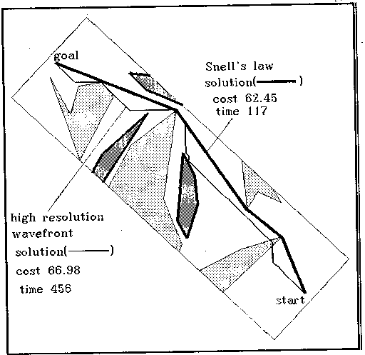
Figure 15
Special-purpose hardware (Parodi 1985; Witkowski 1983) speeds wavefront propagation significantly, but special-purpose hardware can speed our algorithm too. Tree-structured processor architectures (Shaw 1987) could help: upon each wedge partition, a different processor can be assigned to each wedge. Search processes are central in artificial intelligence, and there has been significant hardware research lately concerning them. In addition, vector-processing hardware can compute line intersections fast, something critical in all parts of our algorithm.
(These tests were done with an implementation designed for terrain with only three kinds of regions: obstacles, high-cost, and low-cost. This reflects our work in planning for tanks in the Point Lobos and Fort Hunter-Liggett terrain, in which this tripartite division follows military doctrine (forests are high-cost and grassland is low-cost). But generalizing our program requires only minor code changes.)
An extension to interpolation regions
One problem with a homogeneous-cost-region representation of terrain is the artificially abrupt index transitions on region boundaries. To better model the real world, we can introduce a new kind of region, a nonhomogeneous "interpolation region" or "spline region" inserted between homogeneous regions of different index, across which the index would vary smoothly with position. Such regions can model the shoulders of roads and the edges of rivers.
Suppose the index is solely a function of the x-coordinate in some
coordinate system. Then (using a trick of Fermat) we can model the terrain as a
set of infinitesimally thin horizontal bands, each with a uniform cost as the
width of the bands approaches zero in the limit. By transitive application of
Snell's Law across the bands, the quantity ![]() is invariant along any optimal
path, where n(x) is the index and θ is its slope angle. If we know the
starting
is invariant along any optimal
path, where n(x) is the index and θ is its slope angle. If we know the
starting ![]() and
and
![]() , we can
rearrange the differential equation to calculate y for the path as a function
of x:
, we can
rearrange the differential equation to calculate y for the path as a function
of x:
A simple application of the above integral is to a region in which the index
at any point is ![]() where
x is the distance across the region; note this is a monotonic function of x. If
a rectangular such region of width W interpolates between regions of indices
where
x is the distance across the region; note this is a monotonic function of x. If
a rectangular such region of width W interpolates between regions of indices ![]() and
and ![]() , then
, then ![]() . Then the above
integral gives a circular arc whose direction at
. Then the above
integral gives a circular arc whose direction at ![]() is perpendicular to the boundaries.
So if we are given the region-entering angle
is perpendicular to the boundaries.
So if we are given the region-entering angle ![]() of a path, the region-leaving angle of
the path is given by
of a path, the region-leaving angle of
the path is given by ![]() ; the place of leaving can be determined
from the radius of curvature,
; the place of leaving can be determined
from the radius of curvature, ![]() . This means that wedges crossing such
interpolation regions are bent so that their boundaries are circular arcs of a
computable curvature. Figure 16 gives an example in which the dark region in
the center represents a road, and the shaded regions to the left and right of
it represent shoulders interpolating between a background region of twice the
cost of the road. Curved wedges complicate details such as the calculation of
upper and lower cost bounds, but our algorithm can use them and remain
fundamentally the same.
. This means that wedges crossing such
interpolation regions are bent so that their boundaries are circular arcs of a
computable curvature. Figure 16 gives an example in which the dark region in
the center represents a road, and the shaded regions to the left and right of
it represent shoulders interpolating between a background region of twice the
cost of the road. Curved wedges complicate details such as the calculation of
upper and lower cost bounds, but our algorithm can use them and remain
fundamentally the same.
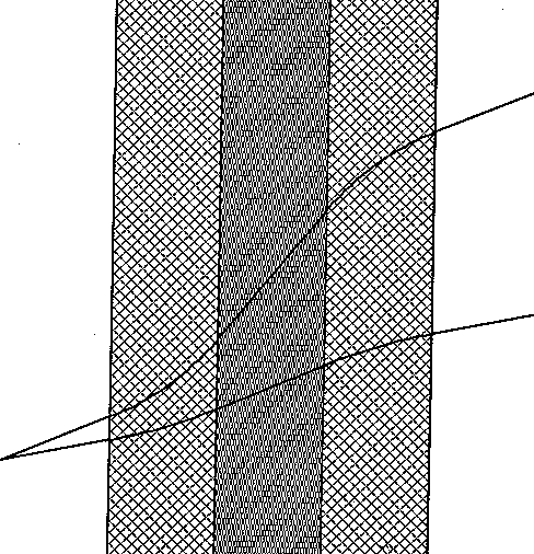
Figure 16
Conclusion
Our approach to path planning finds optimal paths in an intelligent, natural way. It systematically exploits optics analogies to reduce the problem to finite A* search, whereupon a variety of pruning criteria can provide search efficiency. Our method has advantages over the traditional wavefront-propagation methods because one can model the world better with irregularly-shaped regions than with a uniform grid. It can thus (1) find paths closer to optimal; (2) solve conceptually simple problems quickly, sometimes dramatically so, avoiding obvious useless search directions; (3) avoid unreasonable jagged paths due to digital approximation; (4) reduce roundoff errors; and (5) avoid directional bias in paths. Furthermore, our method is considerably more efficient in the average case than the only other Snell's Law algorithm proposed for path planning. We thus expect it to be a valuable tool in the arsenal of spatial-reasoning methods.
References
Brooks, R. A. 1983 (March/April). Solving the find-path problem by good representation of free space. IEEE Transactions on Systems, Man, and Cybernetics SMC-13(3): 190-197.
Chavez, R. and Meystel, A. 1984 (Atlanta, Georgia). Structure of intelligence for an autonomous vehicle. Proceedings of the International Conference on Robotics. New York: IEEE, pp. 584-591.
Crowley, J. L. 1984 (December, Denver, Colorado). Navigation for an intelligent mobile robot. First IEEE Conference on Artificial Intelligence Applications. New York: IEE, pp. 79-84.
Graglia, P. and Meystel, A. 1987 (Philadelphia, Penn.). Planning minimum time trajectories in the traversability space of a robot. Proceedings of the IEEE International Conference on Intelligent Control. New York: IEEE.
Lozano-Perez, T. and Wesley, M. A. 1979 (October). An algorithm for planning collision-free paths among polyhedral obstacles. Communications of the ACM 22(10): 560-570.
Kambhampati, S. and Davis, L. S 1986 (September). Multiresolution path planning for mobile robots. IEEE Journal Of Robotics And Automation RA-2(3): 135-145.
Metea, M. B. and Tsai, J. J.-P. 1987 (February, Raleigh, North Carolina). Route planning for intelligent autonomous land vehicles using hierarchical terrain representation. Proceedings of the 1987 IEEE Conference On Robotics And Automation. New York: IEEE, pp. 1947-1952.
Mitchell, J. S. B. 1988. An algorithmic approach to some problems in terrain navigation. Artificial Intelligence 37: 171-201.
Mitchell, J. S. B. and Papadimitriou, C. H. 1990. The weighted region problem. Journal of the ACM, to appear.
Mitchell, J. S. B., Payton, D. W., and Keirsey, D. M. 1987. Planning and reasoning for autonomous vehicle control. International Journal of Intelligent Systems 11: 129-198.
Parodi, A. M. 1985. Multi-goal real-time global path planning for an autonomous land vehicle using a high-speed graph search processor. Proceedings of the IEEE Conference on Robotics and Automation. New York: IEEE, 161-167.
Richbourg, R. F. 1987 (June). Solving a class of spatial reasoning problems: minimal-cost path planning in the Cartesian plane. Ph. D. Thesis, U. S. Naval Postgraduate School, Computer Science Department. (Also Technical Reports NPS52-87-021 and 022.)
Richbourg, R. F., Rowe, N. C., Zyda, M., and McGhee, R. B. 1987 (February, Raleigh, North Carolina). Solving global two-dimensional routing problems using Snell's Law and A* search. Proceedings of the 1987 IEEE Conference on Robotics and Automation. New York: IEEE, 1631-1636.
Rowe, N. C. 1988. Artificial Intelligence through Prolog. Englewood Cliffs, New Jersey: Prentice-Hall.
Rowe, N. C. 1989. Roads, rivers, and obstacles: optimal two-dimensional route planning around linear features for a mobile agent. International Journal of Robotics Research, to appear.
Rowe, N. C. and Ross, R. S. 1988 (November). Optimal grid-free path planning across arbitrarily-contoured terrain with anisotropic friction and gravity effects. Technical report NPS52-89-003. Monterey, California, USA: U.S. Naval Postgraduate School, Department of Computer Science.
Rueb, K. D. and Wong, A. K. C. 1987 (March). Structuring free space as a hypergraph for roving robot path planning and navigation. IEEE Transactions on Pattern Analysis and Machine Intelligence PAMI-9 (2): 263-273.
Rula, A. A. and Nuttall, C. J. 1971 (July). An analysis of ground mobility models (ANAMOB). Technical Report M-71-4. Vicksburg, Miss.: U.S. Army Corps of Engineers, Waterways Experiment Station.
Shaw, D. E. 1987 (March). On the range of applicability of an artificial intelligence machine. Artificial Intelligence 32 (2): 151-172.
Thorpe, C. E. 1984 (August, Austin, Texas). Path relaxation: path planning for a mobile robot. Proceedings of the National Conference on Artificial Intelligence. Menlo Park, Cal.: AAAI, 318-321.
Turnage, G. W. and Smith, J. L. 1983 (September). Adaptation and condensation of the Army Mobility Model for cross-country mobility mapping. Technical Report GL-83-12. Vicksburg, Miss.: U. S. Army Corp of Engineers, Waterways Experiment Station.
Witkowski, C. M. 1983 (August, Karlsruhe, West Germany). A parallel processor algorithm for robot route planning. Proceedings of the Eighth International Joint Conference on Artificial Intelligence Palo Alto, Cal.: William Kauffman, pp. 827-829.
Appendix: The cost convexity theorem
We prove over the set of all paths between some start and goal points that cross the same region-boundary edges in the same order, assuming homogeneous isotropic regions with a uniform cost per unit distance, that path cost is a convex function of parameters necessary to specify the path. For these parameters, take the distances along the region-boundary edges from some fixed points. We will show that each subcost of the subpath between region boundaries is convex; the sum of convex functions is convex, so the total cost is convex.
First consider the beginning and ending segments of the optimal path. Let |x| represent the distance along the first or last region boundary from the projection of the start or goal point onto its line extension, and assume this projection has length |c|. The cost between the start or goal and this boundary is |sqrt { x sup 2 + c sup 2 }| which has a second derivative with respect to every other variable besides x of zero, and with respect to x of |c sup 2 ( x sup 2 + c sup 2 ) sup -1.5 |, a nonnegative quantity.
For all other path segments, first assume the two boundaries are not parallel, and let |x| and |y| be distances along the lines containing the boundary line segments, distances from the intersection of those lines. The law of cosines says that the subpath distance is |( x sup 2 + y sup 2 - 2 x y cos H ) sup 0.5 |. Convexity is proved from:
lambda ( x sub 1 sup 2 + y sub 1 sup 2 - 2 x sub 1 y sub 1 cos H ) sup
0.5 + ( 1 - lambda ) ( x sub 2 sup 2 + y sub 2 sup 2 - 2 x sub 2 y sub
2 cos H ) sup 0.5
>= [ ( lambda x sub 1 + ( 1 - lambda ) x
sub 2 ) sup 2 + ( lambda y sub 1 + ( 1 - lambda ) y sub 2 ) sup 2 - 2
( lambda x sub 1 + ( 1 - lambda ) x sub 2 ) ( lambda y sub 1 + ( 1 -
lambda ) y sub 2 ) cos H ] sup 0.5
by squaring both sides, cancelling terms, rearranging, squaring again, and cancelling terms to get a nonnegative sum of squares; we skip the tedious details. If the region boundaries are parallel at distance |D|, measure the distances |x| and |y| along them relative to some perpendicular line. Then subpath distance is |sqrt { ( x - y ) sup 2 + D sup 2 }|. Convexity follows from
lambda sqrt { ( x sub 1 - ysub 1 ) sup 2 + D sup 2 } + ( 1 - lambda ) sqrt { ( x sub 2 - y sub 2) sup 2 + D sup 2 } >= sqrt { [ lambda x sub 1 + ( 1 - lambda ) xsub 2 - lambda x sub 2 - ( 1 - lambda ) y sub 2 ] sup 2 + D sup 2 }
which can be shown by the same methods as the general case.
Figure captions
Figure 1: Example in which an irregular terrain representation is better
Figure 2: Example of terrain needing varying resolutions (high-cost regions are shaded, obstacle region is black)
Figure 3: Higher resolution for wavefront propagation doesn't help much
Figure 4: A bad case for hierarchical wavefront propagation
Figure 5: Some Snell's Law paths within the wedge (which is also a WBPS) crossing the four horizontal region boundaries (shaded areas are high-cost)
Figure 6: Two examples of middle wedges when searching from S
Figure 7: Total internal reflection of part of a wedge
Figure 8: Control flow in the algorithm
Figure 9: Example terrain
Figure 10: Example A* search tree
Figure 11: Example ellipse containing start S and goal G (shaded regions are high-cost)
Figure 12: Example for bounds from previously-cached optimal paths (shaded region is high-cost)
Figure 13: An example in which the goal point can fall within many wedges (shaded regions are high-cost)
Figure 14: Statistics on some experiments with our program on an artificial terrain (similar results were obtained for a real terrain)
Figure 15: A simple example illustrating the differences in the paths found by our algorithm and wavefront propagation (note the experiments summarized in Figure 14 were generally more complicated paths than this)
Figure 16: A curved wedge arising from crossing interpolation regions