Change Detection for Linear Features in Aerial Photographs

�Using Edge-Finding

Neil C. Rowe and Lynne L. Grewe (*)

Code CS/Rp, U.S. Naval Postgraduate School

Monterey, CA 93943 USA; rowe@cs.nps.navy.mil

* - Currently with Computer Science Department, California State University,

Hayward, Hayward, CA 94542 USA, grewe@csuhayward.edu

Abstract

We describe a system for automatic change detection of linear features such as roads and buildings in aerial photographs.� Rather than compare pixels, we match major line segments and note those without counterparts.� Experiments show our methods to be promising for images of around 2-meter resolution.

Acknowledgments: This work was sponsored by the U.S. Navy Tactical Exploitation of National Capabilities (TENCAP) program.

This paper appeared in the IEEE Transactions on Geoscience and Remote Sensing, Vol. 39, No. 7 (July 2001), 1608-1612.

1. Introduction

Change analysis between aerial photographs taken at different times is valuable for analyzing the effects of weather, crop diseases, environmental degradation, and expansion of urban centers [7]. Usually this involves subtracting brightness values, in some spectral range, of corresponding pixels [2] to get a "difference image", perhaps with some mathematical adjustment using various local and global features [5, 8], and presenting this graphically to a user with some coding scheme.� This works well for broad-scale (100-meter resolution) images and large-scale changes such as vegetation growth. However, changes of military significance are often more localized, as the changes to buildings and roads that were of particular concern in the 1990s in Iraq and in aerial surveillance of Kosovo in 1999. Military needs often focus attention on changes to straight-line segments -- their appearances, disappearances, size and orientation changes -- and the shapes which the segments form.� So they need edge analysis and shape-recognition techniques [3, 9, 10].� Military applications cannot assume good weather or lighting conditions, so methods must be robust.� Also, many important changes will be on a 5-meter or 2-meter scale and we will need sufficient resolution.

Our approach is to coarsely register two images relative to one another; normalize the brightness and contrast; find edge cells; extract significant line segments; find the best matches of line segments between the images; calculate the pixel-location mapping function between the images; subtract out corresponding segments and edge pixels; and present the "difference" pixels highlighted on the original images to the human intelligence analyst.� The results can also be used to automatically update terrain databases [1].� Matching of edge segments has less sensitivity to changes in illumination, vegetation, and viewing conditions than pixel subtraction does; it permits comparison of quite different pictures like black-and-white with color infrared, like the U.S. Geological Survey images of the United States which alternate every six years between those formats and do not respond well to direct subtraction.� Matching of edge segments can also be made tolerant of small errors in registration due to shadows, perspective, and changes in vegetation and water, thus reducing effects of the important misregistration problem in pixel subtraction [4].

2. Image normalization

For image differencing, it helps if the images are as similar as possible.� We convert color images to grayscale by summing brightness values over all spectral ranges, and normalize the brightness and contrast.� (Normalization has only a minor effect on edge-finding but helps the analyst viewing the output of processed images.)� For this we filter the first image of each pair in the wavelet domain, followed by a 3 by 3 median substitution on both images.� Wavelet transforms are good for normalization because they permit different adjustments on different image scales.� Our initial wavelet normalization is "global", based on parameters of the entire image.� Specifically, the first image is transformed to the wavelet domain, smoothed, multiplied to equate its mean to that of the second image, and transformed back to the image domain.� We also explored "local" normalization which works successively on small corresponding areas of the images, using our calculated fine-grain registration described below; it requires extra time since segment matching must be done twice, but can help accuracy.

3. Registration of image pairs

We assume two aerial photographs roughly covering the same area, taken at different times with not necessarily the same camera, film, or viewing conditions.� We assume that 50% of their area overlaps, their scale differs by not more than 30%, their orientation differs by not more than 0.3 radians, and their obliqueness (angle from directly overhead) is no more than 0.3 radians.� These limits represent our judgement as to what humans would consider a matching pair of images; they also correspond experimentally to limits beyond which our system is inefficient.� Specifications in the metadata of images often guarantee these limits; or a user can enforce them by explicitly matching points in the images, or we can use a known registration for a neighbor image pair, but this research explored what could be done without such extra help.� This leaves a remaining problem of fine-grain registration, necessary for detecting small changes between the images, and desirable to automate since people find it difficult and tedious.� Many good methods can be used, like matching road intersections [6].� But since we need to compare line segments anyway for change analysis, we match them for registration.

3.1 Finding line segments

We use the Canny edge finder [10] to find "edge cells" or pixels between significantly different brightness values.� We preferred the Canny method since it produced longer connected segments than the other algorithms we tried, which helps in matching.� Edge cells are found twice using two thresholds: one yielding about 10% of the image as edge pixels, and a threshold 25% of that.� The first edge image is used for edge matching, and the second only at the last step to rule out borderline edges, edges above the threshold in one image and below in the other.

To find line segments from edge pixels, we calculate the Hough transform [10] (a mapping from pixel locations to possible line equations containing them) of the 10% edge image.� We weight it by the inverse of the corresponding line length lying within the image boundaries, to compensate for the reduced edge-cell opportunities of lines crossing less of the image.� We find the local maxima of the transform array.� Then in descending order of maxima height, we find edge cells within 1 pixel of the corresponding line, and try to find clusters of 10 or more contiguous cells.� Maxima are only considered if greater than the expected number of edge cells if pixels were distributed randomly.� We then discard non-cluster edge pixels, recalculate the transform on the remaining edge pixels, and search again for line segments.� This second pass can find segments confusable with nearby ones found in the first pass, like the parallel line segments of roads.

For each pixel cluster found, we determine endpoints, orientation , and offset D for the least-squares line.� Then since the sign of the contrast rarely changes along a road or building edge (with exceptions such as with long changing shadows, snowfall, and drought), we redefine �on a range of 0 to �where the brighter region lies to the right in the direction of orientation.

3.2 Segment-to-segment matching

We now do fine-grain registration of the two images by matching their edge segments.� However, several matches to the same segment may lie within the coarse-registration tolerance since ground structures often have parallel edges.� Fortunately, several clues can filter out incorrect matches.

We first find good line-segment matches of the 100 longest segments in each of the two images.� The assumption that image rotation is less than 0.3 radians rules out around 95% of possible matches.� We also rule out matches differing more than 2:1 in length; this rules out around 80% of the remaining matches, 90% of the discarded matches being indeed invalid.� Finally, we superimpose the images and measure two factors for each segment pair, "parallel distance" (the distance of the midpoint of the first segment from the line containing the second segment) and "collinear distance" (the distance between the projections of the segments onto the line through the second segment, defined to be negative if the projections overlap).� We limit both factors to 16% of the average length of the diagonal of the two images for this initial matching, ruling out about 68% of the remaining segment matches.� If necessary, we exclude the edges with the most possible matches to reduce the total number of matches to no more than 100, since such edges are the most ambiguous.

Figure 1 shows two example edge images.� Edge 1 of the left image can match either 11 or 13 of the right image, but not 12 because of its orientation.� Edge 6 cannot match edge 12 because it is more than twice as long.� Depending on the accuracy of the superposition and the thresholds, edge 13 can be matched to 3 or 5 but probably not 1 by the parallel distance criterion, and probably not 4 by the collinear distance criterion.

3.3 Matching groups of line-segment matches

We now filter segment matches by considering their consistency.� We start with pairs of segment matches (that is, four segments in two matched pairs).� Correct segment matches will appear in more of the reasonable pairs than incorrect matches will.� We require the rotation angle be consistent within 0.1 radians for a pair; this rules out about 83% of the pair-pair matches.� We also rule out matches with inconsistent scales or angles for their segment pairs, which rules about another 20% of the pair-pair matches.� We then select the best 25% of the pair-pair matches with weighted criteria including segment lengths (pairs with longer segments are more reliable), length consistency, and the distance between the segments in each image (segments further apart provide more accurate estimation of parameters).

Then we consider possible sets of three match pairs ("triples") built from three identified pairs.� We can fit a unique 4-parameter linear mapping from the equations of the six lines through the six segments, avoiding reliance on the possibly inaccurate endpoints: �and .� Here �and �are translational offsets, s is the scale factor, and �is the image rotation.� This assumes images at the same viewing angle, but otherwise the error is usually small, and this assumption is relaxed anyway in the next step.

With this, the line �is mapped to �where �and .� Given three segment-match pairs, we estimate the rotation as average of the three matched orientation differences; substituting this in the line equation yields three linear equations in , , and s.� We solve these, and eliminate triples with fits outside the acceptable ranges of translation, rotation, and scaling.� We also superimpose the segments using the mapping function, and eliminate triples whose collinear distance is nonnegative.� A good triple for Figure 1 would be 1-11, 2-12, and 3-13 because the segments are close enough and different enough in orientation and size to provide good constraints.� Now since we usually have weeded out most incorrect segment matches, we eliminate triples with atypical mapping functions, ones with rotation and scale factors more than 0.1 from the median.� These criteria together eliminate 99.9% of the triples on the average.

We now combine triples to obtain sextuples of matched segments.� This permits a least-squares fit to the general linear mapping between two planes, which can handle arbitrary oblique images: and .� We impose reasonability constraints on matches that 0.7 <a < 1.3, 0.7 <e <1.3, -0.3 < b < 0.3, �-0.3 <d < 0.3, 0.1 < a-e, 0.1 < b-d, and that c and f must be smaller than the half the larger dimension of the corresponding image.� This typically eliminates 99% of the possible sextuples, but there is much variability.

It now likely that the best sextuples correctly match the images. Thus we average the fits for the 200 best-fit sextuples to get a consensus mapping function.� We then map all (not just 100) segments of the first image to the second image using it.� For each segment of the first image, the best possible segment match in the second image is found that obeys the constraints on orientation, size, parallel distance, and collinear distance.� We refit the six parameters using these matches to get our final mapping function.� Optionally, this can be used to better normalize the images by local correction with the wavelet transform.

4. Calculating the edge-difference image

Now we can use our mapping function and segments to create two "edge-difference images", binary images showing the edge pixels that do not correspond to edge pixels in the other image.� To obtain them, we filter edge pixels instead of segments:

1. Edge pixels in either image mapped outside the boundaries of� the corresponding image are eliminated.

2. All pixels of edge segments matched to an edge segment of the other image are eliminated.

3. Edge pixels that map within a pixel of a segment of the other image, or to an edge pixel at the lower (25%) threshold mentioned in section 3.1, are eliminated.� This helps eliminate pieces of broken edges.

4. The remaining edge pixels for each image are clustered into sets of contiguous pixels.� Clusters of less than a minimum size (currently 2) are excluded.

The remaining edge pixels comprise the "on" cells of the edge-difference image.� They are highlighted on the two images and presented to the user for inspection, superimposed in dark black or red on the whitened original images.� A human expert should be able to see patterns of change at a glance.� Figures 2 and 3 show example output for an industrial park in Monterey, California, USA between 1987 (color infrared film) and 1993 (conventional black-and-white film), the first pair listed in Figure 4.� Parts (but not all) of new buildings and cleared areas were found and large vegetation changes were noted.

5. Experimental results

Our program is around 1000 lines of source code primarily in the Matlab language, with wavelet normalization in Java.� Processing averaged 12 minutes for a 256 by 256 image on a Windows NT workstation with a processor having a 2 nanosecond cycle, reasonable for this mostly-uncompiled program; roughly equal time is spent on each of segment finding, fine-grain registration, and building the edge-difference images.� Tables 1 and 2 give processing statistics on representative image pairs extracted from U.S. Geological Survey photographs, where the earlier image was color infrared and the later was conventional black-and-white.� The nonlinearity in the registration mapping averaged 3 pixels for these pairs.� Note that a segment can initially match more than one counterpart.

We measured performance by estimating precision and recall by randomly sampling the output.� Precision was defined as the ratio of the number of "difference pixels" ("on" pixels of the edge-difference images) correctly identified to the number of difference pixels identified; recall was defined as the ratio of the number of difference pixels correctly identified to the number of correct difference pixels.� (Counting pixels rather than segments is better because longer segments matter more than shorter segments.)� Average precision was 0.59 and average recall was 0.54 over the ten tested image pairs with around 8300 correct difference pixels found. In contrast, precision was 0.04 and recall was 0.10 for a control algorithm that eliminates edge pixels matching within a pixel length for the same mapping function, and performance was further worse when manual registration results were used.� Our output should save time for intelligence analysts by focusing their attention.

6. References

[1] W. Baer, L. Grewe, and N. Rowe, "Use of image feedback loops for real time terrain feature extraction," IS&T/SPIE Symposium on Electronic Imaging '99, January 1999.

[2] M. Carlotto, "Detection and analysis of change in remotely sensed imagery with application to wide area surveillance," IEEE Transactions on Image Processing, vol. 6, no. 1, pp. 189-202, January 1997.

[3] R. Collins, C. Jaynes, Y. Q. Cheng, X. Wang, F. Stolle, E. Riseman, E., and A. Hanson, "The Ascender system: automated site modeling from multiple aerial images," Computer Vision and Image Understanding, vol. 72, no. 2, pp. 143-162, November 1998.

[4] X. Dai and S. Khorram, "The effects of image misregistration on the accuracy of remotely sensed change detection," IEEE Transactions on Geoscience and Remote Sensing, vol. 36, no. 5, pp. 1566-1577, September 1998.

[5] K. Greene, B. Kempka, and L. Lackey, "Using remote sensing to detect and monitor land-cover and land-use change," Photogrammetric Engineering and Remote Sensing, vol. 60, no. 3, pp. 331-337, March 1994.

[6] J. W. Hsieh, H. Y. Liao, K. C. Fan, M.-T. Ko, and Y. P. Hung, "Image registration using a new-edge based approach," Computer Vision and Image Understanding, vol. 67, no. 2, pp. 112-130, August 1997.

[7] T. Lillesand and R. Kiefer, Remote Sensing and Image Interpretation.� New York: Wiley, 1987.

[8] J.-.F. Mas, "Monitoring land-cover changes: a comparison of change detection techniques," International Journal of Remote Sensing, vol. 20, no. 1, pp. 139-152, 1999.

[9] B. Nicolin and R. Gabler, "A knowledge-based system for analysis of aerial images," IEEE Transactions on Geoscience and Remote Sensing, vol. GE-25, pp. 317-329, May 1987.

[10] J. C. Russ, The image processing handbook, second edition. Boca Raton, FL: CRC Press, 1995.

Figure and Table captions

Figure 1: Example line segments extracted from aerial photographs in 1987 and 1993 of Salinas, California, USA.

Figure 2: Example output for a 1987 photograph of Monterey, California, USA; dark black points represent edges present in this image but not the 1993 one.

Figure 3: Corresponding output to Figure 2 for a 1993 photograph of Monterey, California, USA; dark black points represent edges present in this image but not the 1987 one.

Table 1: Statistics on the test image pairs: Pair is image pair number, Res is resolution, and Rows and Cols indicate the number of pixels per row and per column of each image.

Table 2: Statistics on processing of test image pairs.� Pair is image-pair number, Segs is number of line segments found in each image, Step 1 shows the number of initial segment matches, Step 2 the number of pairs of matches, Step 3 the number of triples of matches, Step 4 the number of sextuples of matches, Step 5 the number of segment matches after fitting with the sextuple average, Final the final number of matches, Prec (precision) is the ratio of difference pixels correctly identified to those identified, and Rec (recall) is ratio of difference pixels correctly identified to all correct difference pixels.

1

2

4

3

5

6

11

12

13

Figure 1: Example line segments extracted from aerial photographs in 1987 and 1993 of Salinas, CA, USA.

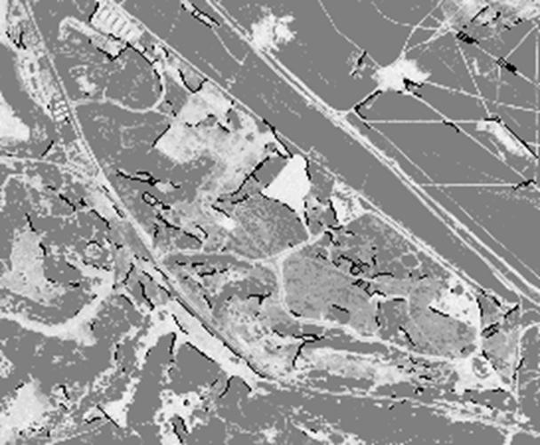
Figure 2: Example output for a 1987 photograph of Monterey, CA, USA; dark black points represent edges present in this image but not in the 1993 one.

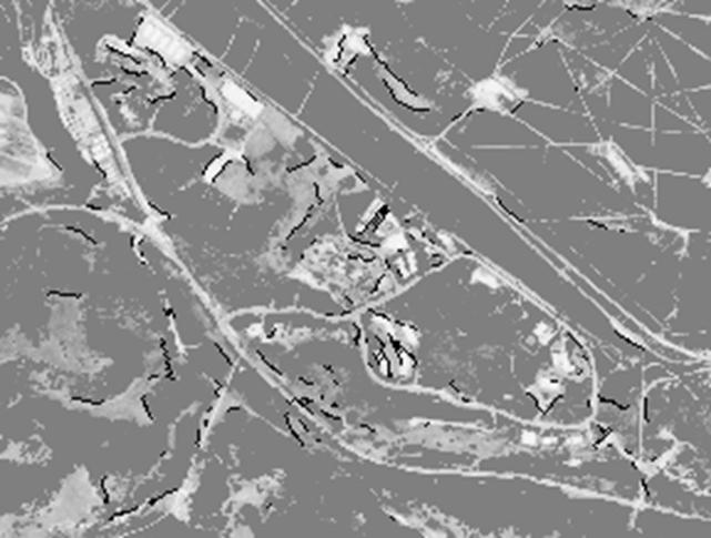
Figure 3: Corresponding output to Figure 2 for a 1993 photograph of Monterey, CA, USA; dark black points represent edges present in this image but not in the 1987 one.

Pair	Type	Res	Rows1	Cols1	Rows2	Cols2
A	Semi-urban	3m.	225	273	218	288
B	Urban	1m.	304	327	304	352
C	Semi-urban	3m.	333	320	344	337
D	Urban	3m.	266	318	233	298
E	Urban	2m.	330	294	313	303
F	Urban	2m.	419	278	443	266
G	Rural	1m.	213	286	207	273
H	Semi-urban	5m.	228	311	255	266
I	Rural	1m.	227	212	254	202
J	Semi-urban	3m.	340	258	277	238

Table 1: Statistics on the test image pairs: Pair is image pair number, Res is resolution, and Rows and Cols indicate the number of pixels per row and per column of each image.

Pair	Segs	Step 1	Step 2	Step 3	Step 4	Step 5	Final	Prec	Rec
A	322 260	260	635	51	28	37	92	0.7	0.4
B	282 352	190	1341	898	11	50	117	0.8	0.5
C	449 392	163	918	423	2305	71	170	0.6	0.6
D	358 253	282	533	43	17	25	55	0.3	0.8
E	492 598	249	996	495	524	73	177	0.5	0.7
F	383 364	320	1269	442	100	79	182	0.6	0.8
G	234 141	259	635	13	5	14	33	0.5	0.2
H	254 264	306	825	65	35	32	88	0.6	0.3
I	254 221	294	933	440	2388	74	154	0.6	0.7
J	385 246	283	1002	493	1379	86	193	0.7	0.4