Approved for public release;
distribution is unlimited
�
Detecting explosive-device emplacement at multiple granularities
July 2010
Neil C. Rowe, Riqui Schwamm, Jeehee Cho, Ahren A. Reed, Jose J. Flores, and Arijit Das
Computer Science, Code CS/Rp, 1411 Cunningham Road
U.S. Naval Postgraduate School
Monterey, California, 93943 USA
ABSTRACT
We report on experiments with a nonimaging sensor network for detection of suspicious behavior related to pedestrian emplacement of IEDs.� Emplacement is the time when detection is the most feasible for IEDs since it almost necessarily must involve some unusual behaviors.� Sensors at particularly dangerous locations such as bridges, culverts, road narrowings, and road intersections could provide early warning of such activity.� Imaging for surveillance has weaknesses in its susceptibility to occlusion, problems operating at night, sensitivity to angle of view, high processing requirements, and need to invade privacy.� Our approach is to use a variety of nonimaging sensors with different modalities to track people.� We particularly look for clues as to accelerations since these are often associated with suspicious behavior.� Our approach involves preanalyzing terrain for the probability of emplacement of an IED, then combining this with real-time assessment of suspicious behavior obtained from probabilities of location derived from sensor data.� We describe some experiments with a prototype sensor network and the promising results obtained.
Keywords: IED, detection, surveillance, sensor, emplacement, acceleration, probability
This paper appeared in the Proceedings of the Military Sensing Society (MSS) National Symposium, Las Vegas, Nevada, U.S., July 2010.
1. Introduction
We are investigating the problem of detecting emplacement of improvised explosive devices (IEDs) in public areas.� Our focus is suspicious behavior by pedestrians using networks of relatively simple nonimaging sensors.� Most previous work has been done with cameras (Bak et al, 2009; Barbara, 2008; Wiliem, 2009).� Cameras are versatile, can detect subtle motion clues such as those indicating deception (Vrij, 2000), and provide data that is easy for personnel to interpret.� But nonimaging sensors have advantages too.� Nonimaging sensors are inexpensive, can avoid problems of occlusion, night and bad-weather conditions, and inconsistencies in performance based on angle of view.� They also minimally invade privacy and require considerably less processing.� Thus they are well suited for monitoring of public areas such as roads.� Nonetheless, they have been little explored compared to camera technology. We have been exploring a variety of sensors (Rowe, Reed, and Flores, 2010), including audio, vibration, infrared, visible-light, magnetic, pressure-strip, and sonar.
Our approach detects suspicious track-related sensor data at three levels of granularity.� Microscale suspiciousness includes overly loud or soft footsteps and those too early or too late after the previous footstep.� Midscale suspiciousness includes inconsistencies in direction, speed, or signal strength.� Macroscale suspiciousness includes appearances, clusters, and speeds inconsistent with cyclic patterns for the day, week, month, or year.� For improvised explosive devices along roads, the latter covers the potential for damage at a given location, the suitability of the terrain for emplacing a device, and the ease of concealment of the emplacement and triggerman.
We report on experiments we conducted with inexpensive sensors in a public place.� The audio and vibration sensors focused on detection of footsteps and used some novel techniques to extract them from background noise.� The other sensors measured close approaches.� Although the individual sensors had both false positives and false negatives, taken together they were surprisingly good, and they did well at detecting suspicious behavior despite missing data.
2. Preanalysis of terrain
2.1. Key principles
A key insight for IED surveillance is that terrain differs considerably in its suitability for an IED:
- Adversaries emplace IEDs where targets are most likely to appear (Ziegler, 2009; Atkinson, 2007).� They study traffic patterns and find places of high average target density.� Often these occur on bottlenecks in roads such as bridges and other narrowings of the road.� It is important to look at multiple scales of resolution (Brantingham et al, 2009) and multiple time periods since traffic can be highly variable.
- The suitability of the terrain for emplacement is an important factor.� Since most IEDs in Afghanistan are excavated, the suitability of the ground for excavation is an important factor there, and that means that earth is much better than pavement (Ziegler, 2009).
- Since emplacement is an inherently suspicious activity, aids to its concealment make it more likely as for other criminal activity (Brower, 1980).� These can be occluding buildings or vegetation.
- If the IED is deployed with a trigger wire, as is common in Iraq not Afghanistan, a triggerman will need to be stationed nearby within visual sighting distance.� So only terrain providing concealment for a triggerman within 50-500 feet for extended periods of time will be suitable (Atkinson, 2007).� This is a stronger condition than that of concealment of the IED location.
- Criminal activity occurs more often where quick egress is possible for the criminal (Newman, 1972).� Thus areas of low mobility such as dead-end streets are not favored for IEDs.� Egress can be for both the emplacer and the triggerman.
- Criminal activity more often occurs when the neighboring population is sympathetic to it.� Many kinds of crime are associated with "territories" (Brown and Altman, 1981).� Cultural and political analysis is needed to find these phenomena.
Of these, the first is the most important, and can be efficiently addressed by automated analysis of traffic patterns as we shall describe.� Suitability of terrain for excavation can be automated using algorithms for classification of surface covering.� Concealment and egressability can be calculated using a graphics model of the terrain (especially the buildings) as we have done previously for the analysis of warfighters during training (Rowe, Houde, et al, 2010).� But cultural and political analysis cannot be easily automated.
2.2. Analyzing traffic patterns
To find traffic patterns for a surveillance area, we do video recording over sample time periods from a fixed camera location and view.� This is not always easy to accomplish in rural areas, but can be done with cameras on temporary poles.� We process the video to count the number of people in a grid of evenly placed rectangular bins across the video, as well as computing their average velocity vectors.� To be effective with this approach, the camera placement must be significantly above the ground to see all areas of the terrain, and we should only analyze portions of the view for which the inclination from the camera is below horizontal.� We assumed the terrain was level in our experiments, though this could be relaxed at the expense of more complex mathematics for mapping from the view to the terrain.� Alternatively if detailed video surveillance is too expensive, an expert could estimate this information from map analysis (Parunak, Sauter, and Crossman, 2009; Li, Bramsen, and Alonso, 2009).
Since there is generally little change between two successive frames of surveillance video, our approach to recognizing people is to subtract images from a "background" image computed each minute.� (This will also find moving vehicles, but we avoided those in our experiments to provide a more uniform task on which to test our methods.)� A total period of one minute was chosen for calculating background because significant effects of the movement of the sun can affect pixel-level analysis outdoors over longer periods of time.� The background image we calculate represents the most typical color of each pixel in the video over the minute.� We find it by taking frames at regular intervals covering the period of the video.� For the set of corresponding pixels for these frames, we find the color that is furthest from the others and compute the average color of the others.� In the current implementation, we do this for nine evenly spaced frames: first three groups of three frames (1, 4, and 7, then 2, 5, and 8, and then 3, 6, and 9), and then on the three resulting images.� This has the effect of excluding pixels where people passed in front of the background since those occurrences will be generally rare in a public area where people are generally moving and will involve usually very different colors than the background.� A disadvantage of this approach is that it will miss people that are stationary over the minute of analysis.� But we found this to be rare in our experiments because people generally moved at least a little when they were waiting or loitering (even when seated).
To segment the video frames, we subtract the red-green-blue image vector for each pixel in the frame from the corresponding color vector for the background image for that minute.� We then create a binary image representing points whose color differences were greater than a threshold.� Regions of this binary image greater in size than a threshold (currently 10 pixels) were considered as people.� We calculate their centroids, and then subtract an amount equal to half the number of pixels that a person of average height would extend at that point in the image as decreased by the effects of perspective.� This gives us the estimated location of the person's feet.
We then transform feet locations from the coordinates of the
image to the coordinates of the ground plane.� A key goal was to make setup as
easy as possible when a new area must be surveyed for sensor deployment.� So
mapping between the image plane and the ground plane is done by an
approximation using five parameters: (1) height of the camera from the ground (![]() ), (2) distance on the ground
from below the camera to the top of the image (
), (2) distance on the ground
from below the camera to the top of the image (![]() ),
(3) distance on the ground from below the camera to the bottom of the image (
),
(3) distance on the ground from below the camera to the bottom of the image (![]() ), (4) length on the ground of
the horizontal line segment halfway down the image (
), (4) length on the ground of
the horizontal line segment halfway down the image (![]() ),
(5) fractional location along that line segment from left to right of the
intersection of the y-axis of the coordinate system where the camera is the
origin (
),
(5) fractional location along that line segment from left to right of the
intersection of the y-axis of the coordinate system where the camera is the
origin (![]() ), and (6) the height in pixels
of a person at the center of the image viewed from ground level (
), and (6) the height in pixels
of a person at the center of the image viewed from ground level (![]() ). Then our calculation of the
mapping from the centroid of a region in the image to horizontal coordinate x
and front-to-back coordinate y in the ground plane in feet is:
). Then our calculation of the
mapping from the centroid of a region in the image to horizontal coordinate x
and front-to-back coordinate y in the ground plane in feet is:

Note this incorporates at the end a rotation of the coordinate system in the ground plane since it is useful to have coordinates based on a natural ground coordinate system independent of the camera view.
We then match ground-plane locations between successive images.� We use a difference metric to find the closest match for each region in the successive or previous image.� The factors in the difference metric are centroid location, size in number of pixels, density of the pixels of the region in their horizontal-vertical bounding box, and color.� We include the best match both forward and backward for a region, which allows for two possible matches if the best match for region R from frame I to frame I+1 (call it R+1) is not the same as the best match from R+1 in the second frame to the previous frame.� This permits regions to split or merge, as can happen when people are wearing different colors on their tops and bottoms and segmentation is inconsistent.� If we cannot find a sufficiently close match for a region, we add a "null-match" hypothesis that it was either created or deleted.� Null matches occur with people far from the camera or people occluded by vegetation or buildings.
We then fit the matches into tracks.� A track must start with a creation event and end with a deletion event.� A track can involve multiple regions, which if they do not get far apart can be considered as two parts of the same person, and we can take their mean location to get the person's location.� A track should generally have a consistent velocity vector.� Exceptions are at splits and merges where two people cross or diverge, and for suspicious behavior.
Figure 1 shows an example background scene created for a video, and Figure 2 shows the locations in the ground plane of people detected.� Figure 3 visualizes the counts in bins of 10 feet by 10 feet (with the area of each circle indicating its count), and Figure 4 shows the average velocity vectors.� The key parameters were measured by tape measure with confirmation from building and landscaping plans.� It can be seen that people are more frequent and more consistent in their directions in the path at the bottom of the image, so this is the most appealing area to emplace a bomb.
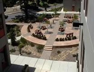
Figure 1: Example synthetic background created from a video.
Figure 2: Track locations of people in a video at noon for the scene in Figure 1.

Figure 3: Visualization of bin counts for terrain in Figure 2 for 10 foot by 10 foot bins.
Figure 4: Average velocity vectors for the video in Figures 1-3.
2.3. Effects of time on traffic
Traffic analysis was done at different time periods to compare traffic patterns over time.� At our school where we did most of our experiments, there are hourly patterns, time-of-day patterns, weekly patterns, and yearly patterns.� Our experiments showed these patterns were quite independent of one another.� This means that we can model the Poisson arrival rate of a person in a bin as a product of factors.� This corresponds to theories of cycles in human and animal activity (Refinetti, 2005).
Calculation of average velocity vectors for people in each bin of the camera view is important in recognizing atypical paths such as loitering.� However, people tend to follow traffic patterns in both directions, and a raw average of their velocity vectors would tend to cancel out motions in both directions.� So as a simple trick, we take the average of the vectors with the same magnitude as the velocity vectors observed but twice the angle from zero orientation, then compute the average vector with half the angle of the computed average.� This then sums together vectors that are 180 degrees apart.
3. Using the sensors
We explored a variety of sensor modalities to test what kinds of sensors were appropriate for the IED-detection task.� The sensors were run off a set of laptop computers in our experiments.� However, there are several lower-cost ways to deploy such sensors in a wireless network (Zhao and Guibas, 2004).� In an environment such as Afghanistan, the sensors and the processors will need to be concealed such as by burying to reduce vandalism.
A variety of clues to suspicious behavior have been proposed (Fong and Zhuang, 2007).� Our previous work has analyzed clues to suspicious behavior, and found that the most useful concerned significant changes to the velocity vector (accelerations) on any of several time scales (Rowe, 2008).� Changes can be in speed or in direction.� Thus our work focuses heavily on tracking people, though other clues to suspicious behavior such as odd footsteps (Itai and Yasukawa, 2008) are useful too.�
3.1. Audio analysis
We also used microphones with Icicle preamplifiers attached to laptops.� Some of the microphones were standard Sony cardioid microphones such as used for music recording, and some like the AudioTechnica AT8804L were intended for radio and had broader sensitivity to the angle of incidence.� Microphones were fitted with wind baffles to reduce the effects of wind noise.
Signals were bandpass-filtered to obtain a range of about 20 to 80 hertz since that seemed to be the most useful range for audio footsteps (though not for seismic footsteps as obtained from the vibration sensor).� Positive peaks around 0.05 seconds in width were found in the resulting signal, and their widths and skews were calculated to aid in matching between microphones; they were then smoothed to reduce the number of spurious peaks.� We only looked for positive peaks because the audio phenomena of interest are generally percussive, involving one object hitting another, and this will usually generate a strong positive peak before a negative one.� Given the average footstep rate of a single pedestrian and the likelihood that around half of the peaks were spurious, we looked to obtain 2.6 peaks per second.� To accomplish this, we decreased the threshold for identifying peaks if the number was too low, and increased it if the number was too high, until we obtained roughly the desired number of peaks per second.� Figure 5 shows a typical resulting signal for three people walking by the microphone (times 240-256, 256-277, and 277-290).� Time synchronization with the sensor readings between microphones was achieved by accessing a time server remotely.� This could alternatively be done in a deployment by using a synchronization signal.
Figure 5: Example footsteps from processing of audio of experiment 6/24/10 from second 240 to second 290.
We use a standard inverse-square model for relating peak
heights to distance, with an additional cardioid dependence of received peak
strength on angle of incidence on microphone.� The model is ![]() �where i is the index of the
sound,
�where i is the index of the
sound, ![]() �is its perceived strength,
�is its perceived strength,![]() �is the intrinsic strength of
the signal i, c is the microphone orientation sensitivity,
�is the intrinsic strength of
the signal i, c is the microphone orientation sensitivity, ![]() �is the bearing of the sound i in
the ground plane,
�is the bearing of the sound i in
the ground plane, ![]() �is the orientation of
the microphone in the ground plane, and
�is the orientation of
the microphone in the ground plane, and ![]() �is
the distance of the sound from the microphone.� The value of c for the Sony
microphones on unobstructed ground as determined by experiments was roughly
0.59 and for the AudioTechnica microphones was 0.61.� We preferred the latter
microphones and did most of our later experiments with them.� This model must
be modified, however, in the case of terrain with many reflecting surfaces.� In
experiments on the floor of a small (18 feet by 12 feet) office, we found that
the average variation with angle was significantly less due to echoes, perhaps
the equivalent of c=0.8, and there were mild asymmetries due to locations of
walls.
�is
the distance of the sound from the microphone.� The value of c for the Sony
microphones on unobstructed ground as determined by experiments was roughly
0.59 and for the AudioTechnica microphones was 0.61.� We preferred the latter
microphones and did most of our later experiments with them.� This model must
be modified, however, in the case of terrain with many reflecting surfaces.� In
experiments on the floor of a small (18 feet by 12 feet) office, we found that
the average variation with angle was significantly less due to echoes, perhaps
the equivalent of c=0.8, and there were mild asymmetries due to locations of
walls.
We can further assume that unsuspicious pedestrians usually
follow straight paths at a constant velocity..� Then �![]() �where
�where ![]() is the distance of nearest
approach of the path to the microphone, v is the velocity of the pedestrian,
is the distance of nearest
approach of the path to the microphone, v is the velocity of the pedestrian, ![]() �is the current time, and
�is the current time, and ![]() �is the time when the pedestrian
approaches most closely to the microphone.� Using four footsteps on a signal
microphone, or two footsteps each on two microphones, we can usually solve for
the location of the pedestrian without using any other sensor data.� If
pedestrians follow a straight path with a constant velocity, we can usually
solve for their path with two footsteps on two microphones.� However, there is
an interesting phenomena with lower values of c that there can be more than one
peak of the signal strength along a straight path.� Figure 6 shows two polar
plots where only the one on the right exhibits this phenomena.� Experimenting
with the parameters of the model, we found that multiple peaks only occurred
for values of c less than 0.57, which was smaller than that of our tested microphone
types, and only for trajectories on the side of the microphone opposite its
direction of orientation for which the signal is weak anyway and thus not
useful.� Thus we ignored this problem in analyzing audio signals, and assumed
that normal straight trajectories demonstrate a single peak of the perceived
signal strength.
�is the time when the pedestrian
approaches most closely to the microphone.� Using four footsteps on a signal
microphone, or two footsteps each on two microphones, we can usually solve for
the location of the pedestrian without using any other sensor data.� If
pedestrians follow a straight path with a constant velocity, we can usually
solve for their path with two footsteps on two microphones.� However, there is
an interesting phenomena with lower values of c that there can be more than one
peak of the signal strength along a straight path.� Figure 6 shows two polar
plots where only the one on the right exhibits this phenomena.� Experimenting
with the parameters of the model, we found that multiple peaks only occurred
for values of c less than 0.57, which was smaller than that of our tested microphone
types, and only for trajectories on the side of the microphone opposite its
direction of orientation for which the signal is weak anyway and thus not
useful.� Thus we ignored this problem in analyzing audio signals, and assumed
that normal straight trajectories demonstrate a single peak of the perceived
signal strength.
Figure 6: Multiple signal-strength peaks can occur with some microphones for straight paths passing the microphone.
Performance of our footstep identification in a sample of 110 seconds in 11 random period during experiments when people were present was 0.19 precision (the ratio of true footsteps in all peaks identified as footsteps) and 0.62 recall (the ratio of true footsteps to all footsteps audible by a person listening to the recording).� Most of the false positives were due to wind gusts despite the microphone baffles; only a few were due to background noise such as motor vehicles and airplanes.� Without people present, we got an average of one false positive every 0.4 seconds with our default parameter settings due to these background noises.� Recall and precision trade off with varying the threshold for peak identification, so precision could be improved at the expense of recall by setting the peak threshold higher.� However, the best threshold depends on the frequency of footsteps in a given area and this can vary considerably.
In identifying "odd" footsteps, we look in particular for unexpectedly loud footsteps, which can indicate sharp turns or abrupt stopping by a pedestrian since strong force is necessary then to counter momentum.� Odd footsteps also occur when people are walking off-road and off-path to avoid IEDs they know about.
3.2. Sensor analysis
For our experiments, we used sensors from Phidgets (www.phidgets.com) and ran them using the Phidget interface hardware (Interface Kit 8/8/8) and software interface (API).� This hardware and software provide an easy plug-and-play environment for testing sensor capabilities, and we could get ten sensors and interface hardware for around $300 at commercial prices.� We laid the sensors mostly on the ground but elevated the sonar and infrared sensors six inches to focus on legs rather than feet and improve detection frequency (see Figure 7).� Sonar, narrow-angle infrared, and vibration sensors were directional and were pointed in different directions to provide broader coverage of human activity.� In Figure 7, the microphone and the sonar sensor on the box point south, the two infrared sensors on the box point west, and vibration sensor points northeast.

Figure 7: Example sensor setup in experiments.
We tested passive-infrared (with a lens), sonar, motion (for diffuse infrared patterns), vibration, magnetic, light-intensity, sound-intensity, and pressure sensors in addition to the microphones.� The infrared and sonar sensors were mounted on boxes about six inches above the ground to focus on legs not feet.� The vibration sensors were either sheltered or enclosed in small boxes to minimize wind effects.� The pressure sensors were placed underneath mats in the center of paths.
Overall the motion sensor was the most helpful for our task, with the infrared and sonar sensors also good.� The motion sensor could pick up approaches within 18 feet in all directions, whereas the infrared and sonar sensors were limited to a sector of about 90 degrees.� The infrared sensor could however detect stationary people which the motion sensor could not.� The (inexpensive) sonar sensor could detect distances to objects in the range of 2 to 20 feet, but produced a noisy signal that required smoothing over time to be useful.� The pressure sensors were useful when they reported something, but they were only an inch wide and four feet long, and people could easily step over them or go around them.� The vibration sensors picked up many spurious signals, even when enclosed in small boxes.� The magnetic sensors only seem to respond to magnetized material, not ferromagnetic material, and were rarely triggered.� The light-intensity sensors saturated quickly in an outdoor setting, and required significant filtering material to cut down the amount of light reaching them.� The sound-intensity sensors were redundant with the microphones and not sufficiently sensitive to provide anything additional.� The individual microphone peaks can be treated with other sensors as indicating a person, but accuracy was much improved by rating peaks by the degree to which they participated in a sequence of 2 to 4 other peaks spaced 0.4 to 0.8 seconds apart, good indicators of footsteps (Sabatier and Ekimov, 2008).� We found it improved performance further to combine all microphone data together to get a single estimated location.
Sensor readings were averaged over each second for each sensor to reduce the effects of noise.� For most sensors, we interpreted each average reading that exceeded a threshold for that sensor as indicating the presence of a person.� Exceptions were the sonar sensor, which gave a distance measurement; the light sensor, for which values less than a threshold indicated human presence; and the microphones as explained.� Default thresholds were the mean of the sensor signal plus twice the standard deviation in a representative time period.� However, some thresholds were adjusted if they were provided too many false positives or false negatives.
3.3. Probability and likelihood distributions of location
For each sensor average per second exceeding its threshold, we create a probability distribution over the ground plane for the presence of a person.� This distribution had a spacing of one foot and covered a bounding box of twenty feet around all the sensors.� The distribution for each type of sensor was calculated by experiments with it.� The nondirectional sensors such as the motion sensor provided a symmetric distribution centered on a point.� We modeled this with a plateau area at the center and a linear taper from an inner radius to an outer radius, which were typically 10 feet.� The directional sensors provide sectors of probability radiating from a point; the sonar had a angular width of 90 degrees, and the narrow-range infrared had an angular width of 40 degrees.� The pressure strips provide a distribution in a well-defined small rectangular area.� The sonar and the audio provide rough distance information; thus the sonar distribution looks like a segment of an annulus, and the audio distribution looks like a full but fuzzier annulus off-center from the sensor location.�
When more than one sensor exceeds its threshold in a one-second interval, we add a weighted sum of the probability distributions to get a likelihood distribution.� The weights were generally the precision of the measurement as indicating human presence (for example, 0.65 for microphone peaks).� This did require adjusting each probability distribution to sum to 1, so distributions that were wider had lower values in each cell.� In the case of a single pedestrian, the centroid of this total likelihood distribution is our estimate of their location.� Multiple local maxima of the distribution indicate multiple pedestrians.� We then partition the distribution along the lines of local minima and take the centroids of each region as the locations of the multiple pedestrians.�
We also average the total likelihood distribution with that of the previous second.� An equal weighting on each worked well.� This handles the problem of missing reports for sensors that only report occasionally during a pedestrian transit, such as infrared.� Such averaging was important in our earlier work (Rowe, Reed, and Flores, 2010) with fewer sensors and those that saturated easily.
The succession of centroids of the probability distributions at each second are taken as the track.� Averaging all the sensor information for one second tends to reduce the effects of spurious peaks due to background noise.� To further eliminate effects of background noise, we eliminate all seconds where the centroid would require more than a speed threshold (currently 5 feet per second) to reach from any other centroid within a time gap (currently five seconds).
3.4. Communication of suspicious-behavior reports
Since the goal of this sensor network is monitoring for suspicious behavior, and such behavior is rare, a good design of the network should not involve much communications traffic most of the time.� Analysis of the likelihood distributions of people within a small area (say on a bridge) can be done by connecting sensors to a single processor.� These should be wired connections since the distances are usually not large.� Note that the local sensors should be aimed in as many different directions as possible when they are sensitive to direction, to provide the maximum amount of coverage given cable length limits.
Then the tracks can be computed and significant accelerations along tracks recognized.� When suspicious behavior is recognized, it can be reported to a base station via an antenna.� For this application, base stations in a range of 100-1000 meters are appropriate.� There will also be reports from individual sensors that need to be reported too, such as excavation signals observed by an audio sensor.� Transmitted data can be in the form of a time, a location, a degree of suspiciousness, and the type of activity that has been identified.
3.5. Table lookup for sensor data
Table lookup is useful for reducing computational requirements in the sensor processors.� A set of sensor values can provide a key to a hash table that is computed in advance for a particular configuration of the sensors (their locations and orientations).� It does require a significant amount of storage, but storage is increasingly inexpensive, and the amount required can be adjusted by controlling the granularity of the hash table.� The hash table can be created either by experiment or by simulation.� Since we found our sensors were reasonably predictable, we opted for the simulation approach.
A hash table can be created by simulating the signals of various types and locations of targets, then modeling the characteristics of our sensors, to generate a table of situations and corresponding signals.� Given a set of observed signals in the real world, we round them to the specified granularity necessary for the table, and search the table to find the closest match.� This avoids the difficult problems of inverting complex nonlinear formulae for the mapping between phenomena and signals.
An example is localization based solely on the peak strengths in the audio.� For a set of microphones, we can calculate the signal strengths for a set of evenly spaced locations in the sensor field.� To provide localization independent of the varying loudness of the sound, we can normalize the values by dividing by the largest one (that of the microphone nearest to the signal).� If the microphone response has no dependence on orientation, the problems reduces to one of intersecting circles (Rowe, 2008).� But even if there is a significant cardioid response, the curves are close to circles.� Figure 8 shows an example, the locus of points having a ratio of 0.5 in strengths for two microphones spaced 1 foot apart and pointing in opposite directions with c=0.6.
Figure 8: Locus of points having a signal-strength ratio of 0.5 for two microphones at (0,0) and (1,0) �pointing in opposite directions with c=0.6.
We then need to collect data from the microphones once the sensor network is running.� Despite synchronization using a time server, times between the microphone peaks could deviate as much a second� due to spreading with echoes and other secondary sounds.� We thus found the best match for each peak between pairs of microphones using as a metric the sum of the absolute value of the time difference and the absolute value of the difference in peak width.� Peak width is defined as the average of the heights plus or minus 0.1 seconds to the peak divided by the height of the peak.� Peak width as so defined appeared to be independent of peak height (see Figure 9), and thus provides a useful additional measure of the relatedness of two peaks.� After finding the best matches between the peaks found for a set of microphones, we combine all the results into a single table, leaving gaps with default heights of zero where microphones could not find matches to others.

Figure 9: Audio peak height (horizontal) versus peak width (vertical) on a typical experiment.
Then given an observed set of signal strengths for the inferred same sound, we compute the ratios to the largest, and find the line of the table whose ratios have the minimum least-squared distance from the ratios observed.� The lookup can be made faster by clustering the data, storing clusters separately, calculating means of clusters, and calculating the closest cluster mean for a given set of signal strengths; then we search the file corresponding to the closest cluster.� This estimate will tend to be most accurate when the signal source is between the sensors, and least accurate when all the sensors have a similar bearing and/or distance from it.
Table lookup based on inverse-square signal strengths will give a unique result for four sensors.� That is because the ratio of strengths for two sensors of the same type with no directional sensitivity in the sensors determines a locus of points which is a circle (Rowe, 2008).� Directional sensitivity is minimal with the broad-response microphones we preferred in our experiments, and serves only to distort the shape of the circle a bit..� Then three sensors of the same type give a locus of two points, and four sensors a locus of one point.� (Very rarely will the sensors have equal circles.)� But we can still use the table approach with fewer sensors.
With three sensors of the same type and locus of two points, there are usually additional clues to decide which of the two is the correct one from additional sensors.� We can use the size of the signal strength itself, rather than its ratios, as an additional parameter.� We can conduct experiments with reference sounds to see how strong they are perceived at different distances.� We can also combine data from other kinds of sensors.� Table lookup can be used as well with binary data such as pressure-plate signals or closest-approach infrared signals.� Then the time of the signal relative to others is the important parameter for the table as well as the binary (present or not) parameter.
4. Experiments
We are testing our approach in a series of experiments with both nonsuspicious and suspicious behavior of pedestrians in a public area.� Suspicious behavior we studied included unexpected halts, unexpected turns, putting down objects, picking up objects, excavation behavior, and carrying of ferromagnetic materials.� Figure 10 shows a typical setup and a subject putting down an object during one experiment.
 �
�
Figure 10: Example experiment 6/24/10, setup and run.
Figure 11 shows overall sensor trigger for four experiments:
1. Each of several subjects in turn walks straight across the sensor field without stopping from bottom to top of the map.� Each subject should wait for the next one to finish before starting.
2. Each of several subjects in turn walks into the sensor field, then makes a sharp right-angle turn across pressure strip 2, then continues in a straight line.� Each subject should wait for the next one to finish before starting.
3. Each of several subjects in turn walks into the sensor field and leaves some objects like books at the location indicated by a star on the map.� They then continue walking in a straight path.� Each subject should wait for the next one to finish before starting.
4. Each of several subjects in turn walks into the sensor field, then picks up their objects at the location indicated by a start on the map.� They then make a sharp right-angle turn across pressure strip 2, then continue in a straight line.� Each subject should wait for the next one to finish before starting.
In Figure 11, dots indicate times at which the sensors readings triggered an event record.� Figure 11 was at time 20-150, experiment 2 (after a false start) was time 200-310, experiment 3 was time 350-490, and experiment 4 was 490-600.� Sensor type 2 is a microphone, type 11 is a pressure strip, type 12 is a directional infrared sensor, type 13 is a vibration sensor, type 14 is a broad-direction infrared motion detector, type 15 is a light sensor, type 16 is a magnetism sensor, and type 17 is a sonar sensor.

Figure 11: Summary of sensor data for the experiment 6/24/10.
�
It can be seen that the motion sensors (type 14) were the most helpful at indicating the presence of people.� Though it is hard to see on this graph, the motion sensors exhibited single triggers for the first two experiments, and double triggers for the last two experiments as was expected.� The pressure strip (type 11) confirmed most of these transits but missed a few because it was not wide enough to require people to step on it.� The directional infrared sensors (type 12) malfunctioned.� The microphones (type 2) and the vibration sensors (type 13) picked up some things but generated many false alarms from wind effects.� Though its results are not well depicted on this kind of graph, the sonar sensor (type 17) was helpful.� The light sensor (type 15) and magnetic sensor (type 16) did not give helpful data in these experiments to we tested them to make sure they were working.
Figure 12 shows an example sequence of inferred distributions in this experiment for a person walking south to north through the center of the area shown.� The left image shows a distribution primarily due to audio.� At t=208 two sonar sensors picked up a person nearby, and this distribution began decaying at t=209.� At T=210 a pressure-strip triggered, giving a strong pattern that overrides the other existing patterns.
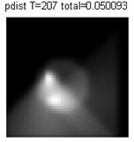


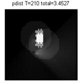
Figure 12: Example probability distributions derived from the data for the 6/24/10 experiment.
Inferred locations can be tracked over time, and velocity and direction changes are straightforward to see. Figure 13 shows an example of an unsmoothed track created from the centroids of 30 seconds of probability distributions.� Figure 14 shows an example of the sequences of centroids person making a right turn, with projections in dark blue onto the ground plane.� In Figure 14 the vertical axis represents time, and the other two axes represent position.
Figure 13: Example track derived from unsmoothed centroids over 30 seconds.
Figure 14: Example of a person making a 90 degree left turn in a sensor field.
With this localization, we can assign a relative danger to each period of time by looking up the inferred location in our preanalysis of terrain for suitability for an IED discussed in section 2.� This permits us to track danger as a function of time.� Then overall suspicious can be a metric on this function curve such as the maximum (for recognizing the most serious threats) or the integral divided by time interval (for recognizing the average level of suspiciousness).� We can also assign a relative suspiciousness to location, as exemplified in Figure 15 where the red areas indicate high areas of suspicious activity as computed for the exercise of 7/9/10.
Figure 15: Suspicious behavior areas for the experiment of 6/24/10.
5. Conclusions
We have presented an approach to detection of suspicious behavior associated with IED emplacement that uses a range of inexpensive commercial off-the-shelf nonimaging sensor modalities.� We have shown how preanalysis of terrain can help, and how different kinds of sensors in combination can provide better functional coverage than any single kind of sensor alone using analysis of probability distributions of locations.� Experiments showed that suspicious behavior can be detected with relatively modest and inexpensive equipment, which is helpful for locations such as rural bridges and culverts.� Since IED threats tend to be quite localized, our networks are a promising way to instrument key areas for robust detection of suspicious behavior.
6. Acknowledgements
This work was supported by the U.S. National Science Foundation under grant 0729696 of the EXP Program.� The opinions expressed are those of the authors and do not reflect those of the U.S. Government.
7. References
Atkinson, R., Left of boom.� Washington Post, September 29 � October 3, 2007.
Bak, P., Rohrdantz, C., Leifert, S., Granacher, C., Koch, S., Butscher, S., Jungk, P., and Keim, D., Integrative visual analytics for suspicious behavior detection.� Proc. IEEE Symp. on Visual Analytics Science and Technology, Atlantic City, NJ, USA, pp. 253-254, October 2009.
Barbara, D., Domeniconi, C. Duric, Z., Fillippone, M., Mansgield, R., and Lawson, E., Detecting suspicious behavior in surveillance images.� Workshops of IEEE Intl. Conf. on Data Mining, Pisa, Italy, pp. 891-900, December 2008.
Brower, S., Territory in urban settings.� In Altman, I., Rapoport, A., and Wohlwill, J., Human behavior and the environment, New York: Plenum, 1980, vol. 4, pp. 179-208.
Bolz, F., Dudonis, K., and Schulz, D., The counterterrorism handbook: tactics, procedures, and techniques.� Boca Raton: CRC Press, 2002.
Brown, B., and Altman, I., Territoriality and residential crime: a conceptual framework.� In Brantingham, P. J., & Brantingham, P. J. (Eds.), Environmental Crimonology, Beverly Hills, CA: Sage, 1981, pp. 57-76.
Brantingham, P., Brantingham, P., Vajihollahi, M., and Wuschke, K., Crime analysis at multiple scales of aggregation: a topological approach.� In Weisburd, D., Bernasco, W., and Bruinsma, G., Putting crime in its place: Units of analysis in geographic criminology.� New York: Springer, 2009, pp. 87-108.
Fong, S., and Zhuang, Y., A security model for detecting suspicious patterns in physical environment.� Proc. Third Intl. Symp. on Information Assurance and Security, Manchester, UK, pp. 221-226, August 2007.
A. Itai and H. Yasukawa, Footstep classification using simple speech recognition technique. �Proc. Intl. Symp. on Circuits and Systems, Seattle, WA, pp. 3234-3237, May 2008.
Li, H., Bramsen, D., and Alonso, R., Potential IED threat system (PITS).� IEEE Conf. on Technologies for Homeland Security, Boston, MA, pp. 242-249, May 2009.
Newman, O., Defensible space: Crime prevention through urban design.� New York: Macmillan, 1972.
Parunak, H., Sauter, J., and Crossman, J., Multi-layer simulation for analyzing IED threats.� IEEE Conf. on Technologies for Homeland Security, Boston, MA, pp. 323-330, May 2009.
Refinetti, R., Circadian Physiology, 2nd Edition.� Boca Raton, FL: CRC Press, 2005.
Rowe, N., Interpreting coordinated and suspicious behavior in a sensor field.� Proceedings of the Meeting of the Military Sensing Symposium Specialty Group on Battlespace Acoustic and Seismic Sensing, Magnetic and Electric Field Sensors, Laurel, MD, August 2008.
Rowe, N., Houde, J., Kolsch, M., Darken, C., Heine, E., Sadagic, A., Basu, A., and Han, F., Automated assessment of physical-motion tasks for military integrative training.� Second International Conference on Computer Supported Education, Valencia, Spain, April 2010.
Rowe, N., Reed, A., and Flores, J., Detecting suspicious motion with nonimaging sensors.� Third IEEE International Workshop on Bio and Intelligent Computing, Perth, Australia, April 2010.
Sabatier, J., and Ekimov, A., A review of human signatures in urban environments using seismic and acoustic methods.� Proc. IEEE Conf. on Technologies for Homeland Security, pp. 215-220, May 2008.
Vrij, A., Detecting Lies and Deceit: The Psychology of Lying and the Implications for Professional Practice.� Chichester, UK: Wiley, 2000.
Wiliem, A., Madasu, V., Boles, W., and Yarlagadda, P., A context-based approach for detecting suspicious behaviors.� Proc. Digital Image Computing: Techniques and Applications, Melbourne, VIC, Australia, pp. 146-153, December 2009.
Zhao, F., and Guibas, L., Wireless sensor networks: an information processing approach.� San Francisco: Morgan Kaufmann, 2004.
Ziegler, J., Improvised explosive device (IED) counter-measures in Iraq.� IEEE Intl. Reliability Physics Symposium, Montreal, QC, p. 180, April 2009.