����������� Image
recognition methods are applicable to a wide range of problems in both the
military and civilian world.� A number of techniques have been utilized in
everything from robot assembly lines to identifying tanks in satellite
pictures.� Much of the research thus far, however, has been restricted to
artificially designed problems in which the test images are carefully selected
or constructed.� In order to build a useful combat system, a method is required
which is robust enough to be used on real images.�
����������� The task of identifying
unknown contacts at sea (ships sighted) is currently delegated to trained human
observers.� Personnel must undergo extensive training in order to meet the
Navy�s need for accurate identification.� They must be regularly retrained as
these skills deteriorate quickly.� In addition, human judgment can be biased by
any number of factors.� If a computer system could be designed to reliably and
accurately perform this function, these problems could be significantly
reduced, leading to better and more efficient performance.
This thesis is the
first step in developing an image analysis module for the Maritime Analysis
Recognition Knowledge System (MARKS) proposed by Lt. Matthew Lisowski, USN.�
MARKS is a design for a platform-independent ship-identification system which
will integrate regional data, emitter analysis, and image analysis to provide
fast, accurate classification of unknown contacts.� Each module will provide
confidence ratings for the most likely candidates, which will be combined by
the system to determine the identity of the contact.� The image analysis module
will operate on a database which is pruned by regional information to contain
only nearby ships.� It will then further narrow the choices by comparing an
image of the unknown ship to those in the database, and will return the most
probable identification and a measure its similarity.
Our image analysis
module operates on a screen capture from infrared (specifically,
Forward-Looking Infrared, FLIR) video.� We require the shots to be close to
broadside, and the entire ship must be within the image boundary.� Otherwise,
we attempt to accommodate as much of the normal appearance of the FLIR images
as possible.� System information projected onto the image (such as crosshairs
and range information) is eliminated by the program�s pre-processing phase, and
small variations in location and orientation of the ship are recognized.� We
then construct a feature vector which efficiently represents the important
characteristics of the ship.� This representation is compared to the feature
representations of all the ships in the database using a standard distance
calculation.� The distances between the ship to be identified and those in the
database become the confidence ratings by which the classification can be done.
In this thesis, we
examine the problems of implementing an algorithm for identifying ships from
FLIR video.� We first review the literature pertaining to our topic, then
describe the program we designed as a possible approach to this problem and its
performance.� Finally, we discuss the implications of our work and the
continuing research it suggests.
����������� The task of image
recognition, whether by computer or by human being, can be broken into three distinct
phases.� First, the observer extracts relevant data out of the scene.� This may
include separating foreground from background, registering color and texture,
or locating edges.� Next, semantic information is imposed on the raw data.�
Areas are numbered, angles are measured, features are labeled, and so on.� By
imposing structure, the image is transformed into a set of facts for use in a
third stage of classification.� In this step, the accumulated knowledge is used
to determine the identity or properties of the target object.
����������� Our focus in this
thesis is on the first part of the recognition process.� We use a simple
similarity metric to classify images.� In chapter 6, we give some suggestions
on how our accuracy might be improved by using more advanced techniques in the
analysis and classification stages.
����������� Prior studies on image
recognition have employed an wide range of disparate techniques.� No one method
emerges from this field as generally superior for all problems.�� The most commonly
applied approaches, however, fall into three broad categories.�
Pattern-matching systems search for particular patterns such as shapes or
angles in an image, and use these as a basis for comparison.� A number of
different mathematical transformations can be applied to images, edge images,
or silhouettes to generate a new image in transform space which is easier to
analyze.� The final set of methods includes those which extract information
from properties of the whole input image, such as moment analysis and some uses
of artificial neural networks.
����������� Searching for
particular shapes can be very effective when the image domain is well-defined.
[Ref. 1] presents a method for identifying ships based on the decomposition of
�bumps� on their decks.� The theory is based on the common rule-based training
students are given when learning to differentiate ship classes.� Each class is
defined by the structures it contains and their arrangement on the deck.� This
forms a rule: A given pattern of structures implies that a ship is of a
particular type. Students then memorize all types of structures, and apply the
rules to determine ship types.�
����������� The goals of this study
were to isolate bumps on a ship�s deck and to accurately determine their
identities.� Silhouettes obtained from [Ref. 2] were searched for locations
where the outline made an upward turn.� Each of the areas defined by such turns
was further analyzed in the same way in order to develop a model of the whole
bump.� Finally, the model was identified using a rule-based system.� The
program found and classified the protrusions with an average accuracy of 78%.�
����������� This work could be
easily extended to identify ships from the pattern of bumps.� Another set of
rules could be constructed to determine what class of ship most closely matched
the current configuration of features.� The usefulness of this method is
restricted, however, by its dependence on detailed, clear silhouettes.� A noisy
image, or one in which the edge of the ship was not continuous, could not be
successfully processed.� The time and space required to identify even these few
features also limits the scaleability of the technique.
����������� The Hough transform was
developed to detect straight lines in images.� Its popularity is largely due to
its ability to operate on noisy or incomplete images, which makes it well
suited to our problem.� While we use the transform as an aid in finding
straight lines, it is possible to make direct comparisons in transform space,
as shown in
[Ref. 3].
����������� This study proposed a
method for locating and recognizing arbitrary two- dimensional shapes.�� First,
the features of the shape to be identified are extracted from a training
image.� The shape is placed at a reference position and orientation, and then
the Hough transform is applied.� Peaks in parameter space are identified, and
their pattern is stored.�
����������� To locate the training
shape in a test image, the pattern of peaks in parameter space is computed as
above.� The one-dimensional convolution of angle histograms for the training
and test peak patterns is calculated.� This function�s highest peak gives the
orientation of the shape in the test image.� Once the angle of rotation is
determined, the patterns can be searched for corresponding peaks.� The
translational displacement can also be found by a three-point comparison of
significant peaks.
����������� The proposed method was
able to successfully locate and confirm shapes made up of straight lines,
independent of rotation and translation.� A scale-invariant extension was also
suggested.� A number of other studies have also designed extensions for the
Hough transform [Refs. 4, 5] or methods involving other transforms [Ref. 6] for
various recognition tasks.
�We attempted to
use a similar technique on our FLIR images, but without success.� Calculations
on the raw Hough transform are difficult and computationally expensive to
extend to complex shapes, especially in noisy images with varying scale,
translation and rotation.� Additionally, since we are trying to classify a ship
rather than to find a known shape, the costly matching process would have to be
done for each possible ship type.
����������� In [Ref. 7], an
experimental system for recognizing aircraft from optical images is described.�
The aim of this research was to classify images of military aircraft by use of
rotation-, translation- and scale-invariant functions.� One type of function
which meets these criteria is a moment-invariant.� The authors defined a set of
moment-invariant functions based on the second- and third-order moments of the
image silhouette, and used them for classification.�
����������� Images for this study
were obtained by photographing white model airplanes against a black
background, then applying a thresholding operation to produce a binary image.�
Six types of aircraft were compared using two separate classification methods,
one based on a nearest-neighbor calculation, and the other on probability
estimation using Bayes� Rule.
����������� This system produced
highly accurate results: fewer than 10 of 132 test images were incorrectly
matched.� It also ran quickly in classification mode.� It is much more
difficult, however, to handle more than six classes and it is questionable
whether the method can be extended to use images of objects in natural
contexts.� Current research at the Naval Postgraduate School is applying
moment-invariants to FLIR image identification.� Other work has illustrated the
merits of different entire-image techniques, such as dominant point detection
[Ref. 8] and improved edge-detection [Ref. 9].
����������� Many object recognition
techniques are also applied in other areas of image processing.� The code we
used to find line segments in our images is a modified form of a function from
[Ref. 10].� Although our purpose was very different from that study, we shared
low-level processing issues.�
����������� The proposed system
compares grayscale aerial photographs to views generated from an existing
database.� Images are searched for landmarks, which are used to find a
transformation to map one image onto the other.� Once the images have been
aligned, a differencing technique is used to find regions that have changed
significantly since the database was last updated.�
����������� The segment finding
procedure that we use is part of the differencing function.� Straight lines are
identified and grouped by the objects they represent.� Lines in the new image
that do not correspond to anything in the terrain database provide evidence for
a new structure or road; lines from the database which do not appear in the new
image indicate that some object has been removed.
����������� In trying to design an
algorithm with the potential for use in a combat system, we had to formulate
requirements additional to those of most current recognition systems.� We
wanted our program to run efficiently in the classification phase so that as we
increased the size of the database, identification could still be done in real
time.� The segmentation portion of the program also needed to run quickly.�
Clearly, we could not use artificially generated images since we were trying to
identify ships from real FLIR video.
����������� Our approach was also
unusual in that we combined some of the standard techniques for recognition in
new ways.� To locate the ship in the image, we used edge detection,
thresholding, and our prior knowledge of the domain.� We extracted line
segments by applying knowledge of Hough transform space features to our edge
image.� In the classification stage, we calculated moments and other
statistical features both on line segments and directly on image pixels.� By
employing different methods on different tasks, we hoped to come up with a
better solution than any individual process could provide.
We used a video capture
card to obtain frames from footage taken by the crew of a SH-60B Rapid
Deployment Kit equipped helicopter. The AN/AAS-44V FLIR is mounted on a
springboard at the nose of the aircraft.
Because we used real FLIR
images as our data, we dealt with a number of challenges in the pre-processing
phase.� We limited our samples to pictures in which the entire ship was visible
and centered, and only used near-broadside views.� Even with these
requirements, the scale, position, and orientation of the ship varied
significantly between images.� The quality of the images was not ideal; we
employed techniques to eliminate as much noise and background information from
our samples as possible.� To be cost-effective, an automated identification
system needs to be able to operate on noisy data.
|
|
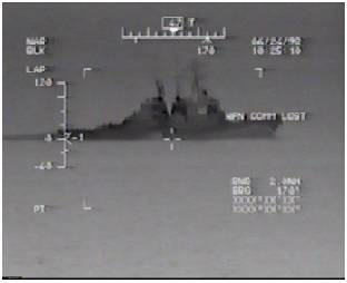 |
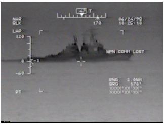
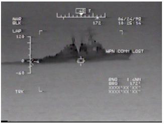
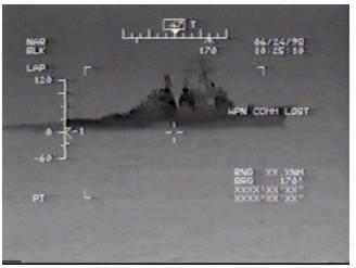
In addition to the problems that always arise when using real data, our images
contained artifacts of the FLIR system from which they were obtained.�� The
system projects video information and targeting aids onto the screen, as shown
in Figure 1.� These may partially obscure the image and interfere with the
identification process.� We tested the efficacy of a number of methods in
removing these factors.
Figure 1.
The FLIR camera
can be operated in a number of modes.� It can display either black-hot (higher
energy areas are black) or white-hot images, and provides both digital and
optical zoom capabilities.� We chose to use only black-hot images because we
can more effectively remove system artifacts from them than from white-hot
images.� We also decided not to allow images produced with the digital zoom
option, as it amplifies background noise significantly.
Our program
operates on images captured from FLIR video using a Studio PCTV.� This system
returns a 320 x 240 pixel TIFF format color image. The program�s second input
argument is a database which contains the comparison information for each
possible ship class.
The program
returns an ordered list of the ships in the database that are closest to the
unknown ship.� Each potential classification has a confidence rating which
represents how similar the test image is to that class.� We list multiple
possibilities because if the test image is very close to more than one database
class, we want the system user to be aware of all strong possibilities.� In the
MARKS system, comparing our results with the results from the emitter and ship
positioning systems will further narrow the database of candidate classes.
����������� We chose to represent
image data as a set of numerical features for three main reasons.� First, we
needed to reduce the amount of data in our comparisons between images if we
wanted to produce an efficient, scaleable system.� We also wanted to make our
program robust enough to operate on real pictures, so we had to find a way to
avoid relying on exact data and to represent general properties of our images.�
Finally, making comparisons based on numbers is much easier than any other
method.� Using numerical features greatly simplified our classification step.�
By extracting important features from the images, we were able to make progress
towards all of these goals.
����������� Using straight line
segments as our basic features fit well with our design objectives.� Ship
images consist mainly of straight lines, so most of the important information
in our images is preserved.� A line segment can also be represented succinctly
by a few numbers: The coordinates of the center, the orientation, and the
length fully describe it.� This choice even helped us to reduce the noise in
the images, as natural noise rarely produces straight lines as long and strong
as those found in man-made objects.
We implemented our program
in MATLAB (version 5.3.1.29215a) using the MATLAB Image Processing Toolbox.�
Because of its extensive image processing toolbox, MATLAB allowed us to
concentrate on the high-level design aspects of the algorithm.� If our
algorithm were used in a real system, it could easily be translated into a more
commonly used language such as C or Ada.
All of our research and
testing were done on a Micron Millennia computer running Windows NT 4.0, so our
run times are all for that platform.�
In order to reduce the
impact of noise on our algorithm�s performance, we combined multiple processing
steps.� During the pre-processing stage, we smoothed the images using standard
median filtering on 3-by-3 pixel neighborhoods.� Filtering reduced the
graininess of the images so that fewer false edges were detected in the next
step of segmentation.� The segmentation process itself eliminated many small
regions of the image that resulted from noise, as we only dealt with line
segments of significant length.�
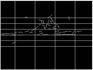
We applied the rest of our
methods after segmentation.� Our limitation to only black-hot images allowed us
to remove all lines from the segmented images which mapped to light areas in
the original images.� Since the heat generated in the engines ensured that the
ship would always be hot relative to the surrounding water, anything �cold�
(light in color) must be noise.� We automatically generated a mask for each
image to represent those pixels with light values, and removed those segments
whose centers were within the mask from the edge image.� This step also removed
some of the processing artifacts, which were generally light.� To deal with any
that remained, we created another binary image that marked all of the areas
where we knew such artifacts would be located.� Then, as above, we disregarded
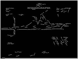
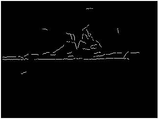
all line segments that fell within those regions.� Figures 2 and 3 show a
segmented edge image before and after these processing
steps.
����������������������������������������������� ������� Figure 2.
������� Figure 3.
����������� We tested and discarded
a few other techniques for the removal of spurious edges. Neighborhood
averaging of light-colored pixels in the original intensity image, which we
hoped would eliminate many spurious edges, did not accomplish anything useful.
We tried smoothing areas that were part of a similar mask to the one discussed
above, also without success.� Finally, we tried to subtract the mask from the
edge image before the segmentation step, with the result that we were unable to
detect many key segments.� Since none of our attempts to clean up the images
before segmentation were successful, we were forced to apply the
post-processing techniques discussed above.� These required additional
processing of the segment list as well as of the resulting image; fortunately,
the impact on program efficiency was minimal.
����������� After converting an
image to grayscale and smoothing it, we searched for strong candidate line
segments to use in classification.� First, we ran the image through an edge
detector.� This process determines which pixels in a grayscale image are on the
boundary between two significantly different shaded regions.� It returns a
binary image the same size as the original image showing the locations of all
edge pixels.� We chose to use the Canny method for edge detection because it
successfully found all of the important features in our images.� We allowed
MATLAB to automatically select the threshold for deciding whether or not a
value change was significant.�
����������� Once all the edge
pixels were located, we began the task of finding connected lines in the binary
images.� For this step, we used a modified version of the segment finding code
from [Ref. 10].� This technique used the radon transform, a version of the
Hough transform, to detect straight lines.� A peak in transform space maps to a
line or lines in image space.� See Appendix B for an explanation of the
mathematics behind this technique.� We found the peaks in the transform, which
gave us the orientation of the strongest lines and their perpendicular
distances from the center of the image.�
����������� When we had this
information, we could find pixels on the lines corresponding to each peak, and
connect pixels using the angle defined by the transform results.� For each
peak, we collected all of the pixels that we reached by simply looking for the
next one nearby and at the correct angle.� Each of these sets approximated a
line segment.� We ran this process twice, first with a higher threshold to
extract major lines, and then again with a lower threshold to find smaller
segments from the pixels which were not matched in the first pass.� After this
step, we had an image made up of numbered straight-line segments and a list of
the endpoints, orientations, and lengths of each segment.
����������� When all of the
segments had been located, we applied the delayed pre-processing methods
described in Section B to eliminate spurious edges caused by noise or FLIR
projection information.� This cleaned up both the image and the segment list.�
As part of this phase, we also determined the center coordinates of each
segment, which we used later for statistical calculations.� Next, we checked
the orientation of the ship in the image to see if we ought to realign it.� We
used the radon transform for this step as well.� Since the highest peak in
transform space usually is the bottom of the ship because the waterline creates
a strong straight edge, we looked at the orientation of that line and rotated
the image to make it horizontal.�
����������� Finally, we removed any
line segments that were on the edges of the image, as they are unlikely to be
part of the ship and would interfere with our statistics.� We found the y-axis
standard deviation of edge pixels, and simply removed any line segments that
fell more than two and a half standard deviations from the image�s y-axis
mean.� The resulting binary image showed the important features of the ship
with very few confounding factors.
|
|
 |
����������� We calculated some simple statistics on the processed images to
help us extract important features.� To account for scale and translation
between images, we first found the median and standard deviation of pixel
locations for both x- and y-axes.� Using this, twenty-five rectangular areas in
the image were defined.� The width of each area was one standard deviation as
calculated along the x-axis, and the height was one standard deviation along
the y-axis.� We centered the first rectangle on the median image pixel, then
added two more rows and columns in every direction, as shown in Figure 4.���
�������
Figure 4.
For each of these ranges, we
counted the number of pixels and then divided by the total number of edge
pixels in the image.� These measures gave a five-by-five array of fractions and
showed how the pixels were distributed and thus gave the approximate shape of
the ship.� Next, we totaled the pixels in each box based on orientation.� We
defined four angle ranges, and for each area, counted the number of pixels
which belonged to line segments in each angle range.� Again, we divided the
results by the total number of image edge pixels.� This step resulted in a
five-by-five-by-four array.� We also calculated the third moment of the image
pixel locations about the mean in the x and y directions (see Appendix B.)�
This feature measures skew or asymmetry, so it was helpful in distinguishing
ship classes such as tankers and destroyers.� The final form of our feature
vector consisted of the two distribution arrays and the moment value, and
contained a total of 126 elements.
To compare two
segmented images, we first calculated the features described above.� Next, we
summed the absolute values of the differences between corresponding features of
the two images.� We used feature weights of 1, 10 and 5 for the pixel
distribution, pixel orientation, and moment differences.� These weights were
chosen subjectively.� The smaller the weighted sum of the absolute differences,
the more alike the two images were judged.�
����������� We had a limited set of
FLIR images for use in our tests.� Consequently, we were not able to experiment
with many different ship classes.� Some of the images we did receive were too
poor in quality to give good results.� Our better images were of Arleigh Burke
class destroyers and aircraft carriers.� We had nine images of Arleigh Burkes
and six images of carriers.� Within those sets, the images varied enough to
make identification difficult.� In order to have more variety in our
comparisons, we included two pictures of Spruance class destroyers in which the
ships were small, as well as one very noisy picture of an Iranian PTG patrol
craft.
����������� In our first trial, we
computed the difference between each of our images separately.� For each image,
we found the feature difference from each other image.� The results from this
test are shown in Table 1.� Since the difference function is commutative the
table is symmetric about the diagonal.� The difference between an image and
itself is always zero, so those entries are left blank.� Smaller differences
indicate images which are more alike.
����������� Table 2 summarizes the
information in Table 1.� For each image, we give the average difference between
that image and the Arleigh Burke images, the carrier images, the Spruance
images, and the patrol craft image.� We also list the minimum image
difference and the image that
produced it.� The averages are taken over all images except the image to which
they are being compared.
|
|
AB avg
|
C Avg
|
DD Avg
|
PTG
|
Min
|
Min Ship
|
|
AB1
|
39.14
|
61.14
|
54.01
|
92.10
|
20.84
|
AB7
|
|
AB2
|
40.76
|
55.45
|
63.76
|
105.09
|
31.69
|
C1
|
|
AB3
|
53.01
|
42.00
|
90.36
|
129.51
|
31.12
|
C3
|
|
AB4
|
60.61
|
86.79
|
50.54
|
63.69
|
41.60
|
AB7
|
|
AB5
|
41.29
|
41.33
|
77.30
|
118.03
|
26.14
|
AB9
|
|
AB6
|
37.33
|
45.75
|
70.34
|
110.36
|
19.50
|
AB9
|
|
AB7
|
36.69
|
60.26
|
52.12
|
92.27
|
20.84
|
AB1
|
|
AB8
|
40.45
|
56.45
|
54.13
|
93.55
|
24.91
|
AB7
|
|
AB9
|
38.50
|
47.29
|
73.69
|
113.25
|
19.50
|
AB6
|
|
C0
|
57.71
|
41.37
|
94.01
|
129.78
|
21.73
|
C3
|
|
C1
|
41.22
|
55.90
|
60.64
|
100.12
|
30.61
|
AB8
|
|
C2
|
44.73
|
40.15
|
76.92
|
112.81
|
26.54
|
AB5
|
|
C3
|
57.30
|
40.07
|
90.32
|
127.28
|
21.73
|
C0
|
|
C9
|
49.15
|
43.03
|
71.31
|
116.65
|
26.91
|
C2
|
|
C10
|
80.86
|
60.50
|
113.41
|
151.81
|
48.61
|
C3
|
|
DD1
|
83.33
|
107.77
|
68.44
|
44.52
|
43.57
|
AB4
|
|
DD2
|
46.95
|
61.10
|
68.44
|
91.57
|
30.59
|
AB8
|
|
PTG2
|
101.98
|
123.07
|
68.04
|
---
|
44.52
|
D2
|
Table
2.
����������� Out of the fifteen
images that were of reasonably good quality (the Arleigh Burkes and the
carriers), eleven (73%) were most similar to another ship in their class.� When
the class differences were averaged, however, thirteen of the fifteen (87%)
were on average more similar to ships in the class to which they belonged.�
This result suggested that when we constructed a database to store data for
multiple ship classes, we should average similarities over many views of the
same ship class to classify a ship.
����������� For another test, we
selected one image from each ship class to put in the database.� We chose the
images that minimized the average difference to the rest of the ships in their
class, using the calculations in Table 2. All of the remaining images were then
compared to these exemplars.� The difference results are shown in Table 3.
|
|
AB7
|
C3
|
DD1
|
PTG2
|
|
AB1
|
20.84
|
66.99
|
75.51
|
92.10
|
|
AB2
|
34.23
|
61.67
|
85.04
|
105.09
|
|
AB3
|
57.41
|
31.12
|
111.77
|
129.51
|
|
AB4
|
41.60
|
91.95
|
43.57
|
63.69
|
|
AB5
|
42.29
|
41.40
|
98.62
|
118.03
|
|
AB6
|
34.98
|
48.01
|
91.50
|
110.36
|
|
AB8
|
24.91
|
60.43
|
77.66
|
93.55
|
|
AB9
|
37.29
|
49.22
|
94.54
|
113.25
|
|
C0
|
65.33
|
21.73
|
117.66
|
129.78
|
|
C1
|
34.96
|
55.89
|
84.36
|
100.12
|
|
C2
|
49.68
|
34.20
|
99.36
|
112.81
|
|
C9
|
55.85
|
39.91
|
96.24
|
116.65
|
|
C10
|
90.81
|
48.61
|
135.02
|
151.81
|
|
DD2
|
32.51
|
66.63
|
68.44
|
91.57
|
Table
3.
����������� Of the thirteen
remaining good images (not counting the Spruance), two Arleigh Burkes and one
carrier were incorrectly identified in this test, for a success rate of 77%.�
Since this was lower than the success rate when we averaged the class values in
Table 2, we tried a new strategy.�
����������� We constructed feature
vectors that were the average of the features over all images in each class
with the exception of two test images, AB9 and C10.� We then tested these two
images against the vector averages.� Our results are given in Table 4.
|
|
AB avg
|
C avg
|
DD avg
|
PTG avg
|
|
AB9
|
37.15
|
39.25
|
76.24
|
113.25
|
|
C10
|
85.38
|
62.30
|
115.74
|
151.81
|
Table
4.
We repeated this process for eight
other pairs of images (AB8/C9, AB7/C3, AB6/C2, AB5/C1, AB4/C0, AB3/C10, AB2/C9,
and AB1/C3), building new feature vectors for each test which were averaged
over the images not in the test set.� Table 5 gives these results.
|
|
AB avg
|
C avg
|
DD avg
|
PTG avg
|
|
AB8
|
35.85
|
60.87
|
55.59
|
93.55
|
|
C9
|
50.52
|
39.38
|
73.54
|
116.65
|
|
|
|
|
|
|
|
AB7
|
36.42
|
64.26
|
53.38
|
92.27
|
|
C3
|
59.90
|
33.33
|
92.39
|
127.28
|
|
|
|
|
|
|
|
AB6
|
37.38
|
48.88
|
73.08
|
110.36
|
|
C2
|
46.14
|
34.78
|
78.08
|
112.81
|
|
|
|
|
|
|
|
AB5
|
43.95
|
44.61
|
80.09
|
118.03
|
|
C1
|
30.41
|
57.72
|
61.75
|
100.12
|
|
|
|
|
|
|
|
AB4
|
66.90
|
89.70
|
35.50
|
63.69
|
|
C0
|
55.83
|
34.86
|
95.40
|
129.78
|
|
|
|
|
|
|
|
AB3
|
57.54
|
39.70
|
91.91
|
129.51
|
|
C10
|
88.65
|
62.30
|
115.74
|
151.81
|
|
|
|
|
|
|
|
AB2
|
29.35
|
58.51
|
64.91
|
105.09
|
|
C9
|
50.21
|
39.38
|
73.54
|
116.65
|
|
|
|
|
|
|
|
AB1
|
36.98
|
62.62
|
55.52
|
92.10
|
|
C3
|
60.20
|
33.33
|
92.39
|
127.28
|
Table 5.
����������� Of our fifteen test
images (we only counted each carrier image once even though we compared some of
them twice), twelve (80%) were correctly identified.� One of the mismatches,
however, was with the Spruance class; since there were only two images in that
group and neither was very good, that test was somewhat unfair.� Ignoring it,
the percentage of accurate classifications between Arleigh Burkes and aircraft
carriers was twelve of fourteen, or 89%.
����������� The most time-consuming
portion of our program by far was the extraction of features from the original
images. Each image required approximately 55 seconds for this step.� Table 6
gives some example times in minutes and seconds for feature extraction.�
|
AB1
|
0:55
|
|
AB2
|
0:40
|
|
AB3
|
1:00
|
|
C1
|
0:50
|
|
C2
|
1:00
|
|
C3
|
0:50
|
Table
6.
Constructing a big image-feature
database will therefore be a lengthy process.� Since the database can be put
together offline, this is not a major concern; what matters more is the
program�s speed in recognition mode.� When making 50 image-pair comparisons,
the total time was less than one second, and for 100 comparisons, the time was
still under three seconds.� Thus a single comparison takes around three
hundredths of a second.
����������� Execution time could be
reduced significantly by running our code on a faster computer.� Translating
our MATLAB code into a more efficient language would also give us a speed
advantage.
����������� This project achieved
our major goals: Our segmentation step produces good results for most of our
test images, and the recognition stage runs quickly and efficiently.� We have
certainly created a foundation on which further work can be built.
����������� Our problems in finding
FLIR images to work with limited our ability to fully test the system.� We only
had four types of ships, and in two of those classes the images were unusable
due to noise and scale.� The results from these trials are less meaningful than
they would be if we had more variation in our data set.�
����������� The classification
results were acceptable, but not perfect.� This is to be expected, as we did
not intend to focus on the classification stage.� We designed a very simple
feature space and difference measure to get some idea of whether our segmented
images contained the relevant information to distinguish between ship classes.�
The features were really an approximation of the ships, rather than an accurate
representation.� With so few features, random statistical similarities between
individual images sometimes outweighed general class similarities.� That is
largely why we had so many incorrect identifications in trials where individual
ships were compared.� Averaging features over classes ameliorated this problem
somewhat, but only increasing the number of features can really solve it.
����������� Many areas of this
project could be improved by further work.� Other edge detectors could be
tested to find out how they affect segmentation.� More features could be
extracted to better represent each ship class.� Features could also be
specified at a higher semantic level, as in [Ref. 2] where low-level
information is grouped to identify masts, superstructures, and gun turrets.� A
more advanced difference calculation could improve performance as well.�
Studies such as [Ref. 8] and [Ref. 9] have proposed methods for a fast Hough
transform, which could speed up segmentation significantly.
����������� Another area for future
study might be the construction of the comparison database.� It would be useful
to look at the results of building a database from non-FLIR images, since data
may not be available for all of the ship types we would like to be able to
identify and visual-spectrum images can be sharper.� Finally, our algorithm does
not currently handle images where the ship is very small or there is too much
noise.� A more robust extension that could work for these cases would be
beneficial.��������
APPENDIX A.
[MATLAB SOURCE CODE]
function [BW,mySegs2] = extractFeatures(I);
I = medfilt2(rgb2gray(I));
[BW,T] = edge(I,'canny');
[BW2,T2b] = edge(I,'canny',T*0.25);
load('roi2.mat');
IT = im2bw(I, 0.5);
[BWRows,BWCols] =
size(BW);
[NBW,RBW,Segsfound2] =
hough_and_segment(BW, 0, 0.03*(BWRows+BWCols));
RBW = bwmorph(RBW,'clean');
RBW = remove_small_regs(RBW,
9);
Regssofar =
size(Segsfound2, 1);
[NBW2,RBW,Segsfound3] =
hough_and_segment(RBW, Regssofar, 10);
NBW = NBW + NBW2;
Segsfound = [Segsfound2;
Segsfound3];
temp3 = double(ROI2) +
double(IT);
temp3 = temp3>0;
mySegs =
centersAndEndpoints(Segsfound);
[mySegs2,segnums] =
remainingSegs2(temp3,mySegs);
BW =
drawLines(NBW,segnums);
figure, imshow(BW);
figure, imshow(NBW);
[BW,mySegs2] =
transformImage(BW,mySegs2);
[BW,mySegs2] =
tightenImage(BW,mySegs2);
function NBW = remove_small_regs(BW,Minlength)
% Remove
small regions in a binary image
[CBW,Numregions] =
bwlabel(BW,8);
NBW = BW;
for I=1:Numregions
��� [YL,XL] =
find(CBW==I);
��� if (max(XL)-min(XL))<Minlength
������ if (max(YL)-min(YL))<Minlength
��������� for J=1:size(XL,1)
������������ NBW(YL(J),XL(J))
= 0;
��������� end���������
������ end
��� end
�end
function newSegs = centersAndEndpoints(seglist);
newSegs = [];
s = size(seglist);
for i=1:s(1)
�� x1 = seglist(i,3);
�� y1 = seglist(i,4);
�� x2 = seglist(i,5);
�� y2 = seglist(i,6);
�� centerX = floor((x1 +
x2)/2);
�� centerY = floor((y1 +
y2)/2);
�� slope = seglist(i,1);
�� r = seglist(i,2);
�� numPix =
seglist(i,7);
�� segment = [x1 y1 x2
y2 centerX centerY slope r numPix];
�� newSegs = [newSegs;
segment];
end
function [newsegs,segnums] = remainingSegs2(ROI,
segsfound);
s = size(segsfound);
newsegs = [];
segnums = [];
for i=1:s(1)
�� if (ROI(segsfound(i,6),segsfound(i,5)) == 0)
����� if (ROI(segsfound(i,2),segsfound(i,1)) == 0) |
(ROI(segsfound(i,4),segsfound(i,3)) == 0)�
������ ��newsegs =
[newsegs; [segsfound(i,:) i]];
����� else
�������� segnums = [segnums; i];
����� end
�� else
����� segnums = [segnums; i];
�� end���������
end
function BW = drawLines(NBW,segnums);
s = size(segnums);
BW = NBW;
for i=1:s(1)
�� [x,y] =
find(BW==segnums(i));
�� sx = size(x);
�� for j=1:sx(1)
����� BW(x(j),y(j)) = 0;
�� end
end
function [BWout,segsOut] = tightenImage(BW,segs);
[y,x] = find(BW>0);
mY = round(median(y));
stdY = round(std(y));
s = size(segs);
segsOut = [];
segnums = [];
for i=1:s(1)
�� if (segs(i,6) < mY + 2.5*stdY) & (segs(i,6)
> mY - 2.5*stdY)
����� segsOut =
[segsOut; segs(i,:)];
�� else
����� segnums = [segnums; segs(i,10)];
�� end
end
BWout =
drawLines(BW,segnums);
function [TBW,newSegs] = transformImage(NBW,segs);
BW = NBW>0;
theta = 70:110;
[R,xp] = radon(BW,
theta);
[M,IX] = max(R);
[M2,IX2] = max(M);
thMax = 381 - IX2;
thMax = ((pi/180) *
thMax);
theta = thMax;
TBW = zeros(size(BW));
[x,y,v] = find(BW);
x = x - 160;
y = y - 120;
s = size(x);
s2 = size(BW);
for i=1:s(1)
�� xi =
round(x(i)*cos(theta) - y(i)*sin(theta)) + 160;
�� yi =
round(y(i)*cos(theta)+x(i)*sin(theta)) + 120;
�� if (xi > 0) & (yi > 0) & (xi <
s2(1)) & (yi < s2(2))
����� TBW(xi,yi) =
NBW(x(i) + 160,y(i) + 120);
�� end
end
s3 = size(segs);
newSegs = [];
for i=1:s3(1)
�� %endpoints
�� ns1 =
round((segs(i,1)-160)*cos(theta)-(segs(i,1)-160)*sin(theta)) + 160;
�� ns2 =
round((segs(i,2)-120)*cos(theta)+(segs(i,2)-120)*sin(theta)) + 120;
�� ns3 =
round((segs(i,3)-160)*cos(theta)-(segs(i,3)-160)*sin(theta)) + 160;
�� ns4 =
round((segs(i,4)-120)*cos(theta)+(segs(i,4)-120)*sin(theta)) + 120;
�� %center
�� ns5 =
round((segs(i,5)-160)*cos(theta)-(segs(i,5)-160)*sin(theta)) + 160;
�� ns6 =
round((segs(i,6)-120)*cos(theta)+(segs(i,6)-120)*sin(theta)) + 120;
�� %orientation
� �ns7 = segs(i,7) + theta;
�� if ns7 > 2*pi
����� ns7 = ns7 - 2*pi;
�� end
�� %r
�� ns8 = segs(i,8);
�� %#pixels
�� ns9 = segs(i,9);
�� %segment number
�� ns10 = segs(i,10);
�� newSegs = [newSegs;
[ns1 ns2 ns3 ns4 ns5 ns6 ns7 ns8 ns9 ns10]];
end
��
function [NBW,RBW,Segsfound] =
hough_and_segment(BW,Baseregnum,Houghthresh)
%
HOUGH_AND_SEGMENT Compute Hough transform and segment
% a binary
image; returns residual binary image and a
% list of
segments
% 3 outputs:
Binary image of matches pixels,
% binary image
of residual (unmatched) pixels,
% and list
of segments found.
RBW = BW;
[BWRows,BWCols] =
size(BW);
NBW =
zeros(BWRows,BWCols);
Segsfound = [];
Regnum = Baseregnum;
theta = 0:179;
[R,P] = radon(BW,theta);
[HRows,HCols] = size(R);
R = [flipud(R(:,end-1))
flipud(R(:,end)) R flipud(R(:,1)) flipud(R(:,2))];
R = colfilt(R,[5 5],'sliding','columnIsolateMax',Houghthresh);
R = R(:,3:end-2);
[XDL,XTL,VL] = find(R);
% Note t and
D here are defined differently in radon than in
% segsfound
to come: they are referenced to center of image
TL = (pi/180) *
(91-XTL);
DL = XDL -
((HRows+1)/2);
WL = [];
for I=1:size(TL,1)
�� EPL =
segment_endpoints_in_box(TL(I),DL(I),BWCols,BWRows);
�� W =
round(1000*(VL(I)/(10+distance(EPL(1:2),EPL(3:4)))));
�� WL = [WL; W];
end
Peakinfo = sortrows([WL
VL TL DL XTL XDL]);
Peakinfo =
flipud(Peakinfo(1+end-min([200 size(TL,1)]):end,:));
if ~ isempty(Peakinfo)
�� TL = Peakinfo(:,3);
�� DL = Peakinfo(:,4);��
�� for K=1:size(TL,1)
����� Peaksegs = [];
����� EPL =
segment_endpoints_in_box(TL(K),DL(K),BWCols,BWRows);
����� if abs(EPL(1)-EPL(3)) >= abs(EPL(2)-EPL(4))
�������� SFlag = 0;
�������� Z0 =
round(min(EPL(1),EPL(3)));
�������� Zend =
round(max(EPL(1),EPL(3)));
����� else
�������� SFlag = 1;
�������� Z0 =
round(min(EPL(2),EPL(4)));
���� ����Zend =
round(max(EPL(2),EPL(4)));
����� end
����� [ORXL,ORYL,Z] =
find_clump(RBW,TL(K),DL(K),BWCols,BWRows,Z0,Zend,SFlag);
����� RFlag = 0;
����� while ~RFlag
�������� RFlag =
(Z>=Zend);
�������� [RXL,RYL,Z] =
find_clump(RBW,TL(K),DL(K),BWCols,BWRows,Z,Zend,SFlag);
�������� Dist =
point_cluster_dist(ORXL,ORYL,RXL,RYL);
�������� if Dist<3
����������� RXL = [ORXL; RXL];
����������� RYL = [ORYL;
RYL];
�������� elseif size(ORXL,1) > 9
����������� [FE,NXL,NYL]
= fit_and_extremes(ORXL,ORYL);
����������� if FE(3)>0 & size(NXL,1)>9
�������������� if distance(FE(3:4),FE(5:6))>8
�����������������
Peaksegs = [Peaksegs; FE];
����������������� Regnum
= Regnum+1;
����������������� for I=1:size(NXL,1)
��������������������
RBW(NYL(I),NXL(I)) = 0;
�������������������� NBW(NYL(I),NXL(I))
= Regnum;
����������������� end
��������������
end
����������� end�����������
�������� end
�������� ORXL = RXL;
�������� ORYL = RYL;
����� end
����� Segsfound = [Segsfound; Peaksegs];
����� if ~ isempty(Peaksegs)
�������� NewPeaksegs = Peaksegs;
����� end
�� end
end
function [XL,YL,Z] =
find_clump(BW,T,D,Cols,Rows,Z0,Zend,SFlag)
%
FIND_CLUMP: Finds connected group of pixels in binary image BW
% that lie
along line defined by (T,D).� Z represents the
% coordinate
(X or Y) of greater extent within box.
Z = Z0;
XL = [];
YL = [];
ST = sin(T);
CT = cos(T);
EFlag = 0;
XC = (Cols+1)/2;
YC = (Rows+1)/2;
EFlag == 0;
if SFlag == 0 & Z < Zend
�� while Z <= Zend & EFlag < 2
����� Y =
round(YC-(D/CT)+((Z-XC)*ST/CT));
����� B1 = BW(Y,Z);
����� if Y<Rows
�������� B2 = BW(Y+1,Z);
����� else
�������� B2 = 0;
����� end
����� if Y>1
�������� B3 = BW(Y-1,Z);
����� else
�������� B3 = 0;
����� end�����
����� if ~(B1|B2|B3)
�������� if EFlag == 1
����������� EFlag = 2;
�������� else
����������� Z = Z+1;
������ ��end
����� else
�������� if B1
����������� XL = [XL;
Z];
����������� YL = [YL;
Y];�����������
�������� end
�������� if B2
����������� XL = [XL;
Z];
����������� YL = [YL;
Y+1];�����������
�������� end
�������� if B3
����������� XL = [XL;
Z];
����������� YL = [YL;
Y-1];�����������
�������� end
�������� EFlag = 1;
�������� Z = Z+1;
����� end
�� end
� elseif SFlag == 1 & Z < Zend
�� while Z <= Zend & EFlag < 2
����� X =
round(XC+(D/ST)+((Z-YC)*CT/ST));
����� B1 = BW(Z,X);
����� if X<Cols
�������� B2 = BW(Z,X+1);
����� else
�������� B2 = 0;
����� end
����� if X>1
�������� B3 = BW(Z,X-1);
����� else
�������� B3 = 0;
����� end
����� if ~(B1|B2|B3)
�������� if EFlag == 1
����������� EFlag = 2;
�������� else
����������� Z = Z+1;
�������� end
����� else
�������� if B1
����������� XL = [XL;
X];
����������� YL = [YL;
Z];�����������
�������� end
�������� if B2
����������� XL = [XL;
X+1];
����������� YL = [YL;
Z];�����������
�������� end
�������� if B3
����������� XL = [XL;
X-1];
����������� YL = [YL;
Z];�����������
�������� end
�������� EFlag = 1;
�������� Z = Z+1;
����� end
�� end
end
function D = point_cluster_dist(XL1,YL1,XL2,YL2);
%
Approximate distance between point clusters in the same
% narrow
corridor from the distance between closest pair
% of
endpoints
if (isempty(XL1) | isempty(XL2))
�� D = 1000;��
else
�� EPS1 =
quick_endpoints(XL1,YL1);
�� EPS2 =
quick_endpoints(XL2,YL2);
�� D1 =
distance(EPS1(1:2),EPS2(1:2));
�� D2 =
distance(EPS1(1:2),EPS2(3:4));
�� D3 =
distance(EPS1(3:4),EPS2(1:2));
�� D4 = distance(EPS1(3:4),EPS2(3:4));
�� D = min([D1 D2 D3
D4]);��
end
function EPS = quick_endpoints(XL,YL)
Xmin = min(XL);
Xmax = max(XL);
Ymin = min(YL);
Ymax = max(YL);
if abs(Xmax-Xmin)>abs(Ymax-Ymin)
�� EP1 = Xmin;
�� EP3 = Xmax;
�� for I=1:size(XL)
����� if XL(I)==Xmin���������
�������� EP2 = YL(I);
����� end
����� if XL(I)==Xmax���������
�������� EP4 = YL(I);
����� end�����
�� end
else
�� EP2 = Ymin;
�� EP4 = Ymax;
�� for I=1:size(XL)
����� if YL(I)==Ymin
�������� EP1 = XL(I);
����� end
����� if YL(I)==Ymax ��������
�������� EP3 = XL(I);
����� end
�� end
end
EPS = [EP1 EP2 EP3 EP4];
function isomax = columnIsolateMax(subarray,thresh);
s = size(subarray);
isomax = zeros(1,s(2));
for i=1:s(2)
�� if ((subarray(13,i) >= max(subarray(:,i))) &
subarray(13,i) >= thresh)
����� isomax(i) =
subarray(13,i);
�� end
end
function EPL = segment_endpoints_in_box(T,D,Cols,Rows)
ST = sin(T);
CT = cos(T);
XC = (Cols+1)/2;
YC = (Rows+1)/2;
if abs(CT)>0.001
�� Y0 = YC - (D/CT);
�� YD = ST*(XC-1)/CT;
�� LY = Y0 - YD;
�� RY = Y0 + YD;��
else
�� LY = 10000;
�� RY = 10000;
end
if abs(ST)>0.001
�� X0 = XC + (D/ST);
�� XD = CT*(YC-1)/ST;
�� UX = X0 - XD;
�� DX = X0 + XD;��
else
�� UX = 10000;
�� DX = 10000;
end
PL = [];
if (LY >= 0.99) & (LY <= Rows+0.01)
� �PL = [PL; 1 LY];
end
if (RY >= 0.99) & (RY <= Rows+0.01)
�� PL = [PL; Cols RY];
end
if (UX >= 0.99) & (UX <= Cols+0.01)
�� PL = [PL; UX 1];
end
if (DX >= 0.99) & (DX <= Cols+0.01)
�� PL = [PL; DX Rows];
end
if size(PL,1)>1
�� EPL = [PL(1,:) PL(2,:)];
else
�� EPL = [PL(1,:) PL(1,:)];
end
if size(PL,1)>2 &
distance(PL(1,:),PL(2,:))<0.03
�� EPL = [PL(1,:)
PL(3,:)];
end
function [Answer,NXL,NYL] = fit_and_extremes(XL,YL)
%
Fit_and_extremes: Compute linear regression and endpoints
% for a set
of points represented by X and Y lists
ON = size(XL,1);
[T,D] =
lsfit_points(XL,YL);
ST = sin(T);
CT = cos(T);
NXL = [];
NYL = [];
for I=1:size(XL,1)
�� if abs((-ST*XL(I))+(CT*YL(I))-D) < 1.01
����� NXL = [NXL;
XL(I)];
����� NYL = [NYL;
YL(I)];
�� end
end
N = size(NXL,1);
if N>1
�� if ON<N
����� [T,D] =
lsfit_points(NXL,NYL);
����� ST = sin(T);
����� CT = cos(T);
�� end
�� R = (CT*NXL)+(ST*NYL);
�� Rmax = [R(1) 1];
�� Rmin = [R(1) 1];
�� for I=1:N
����� if R(I) > Rmax(1)
�������� Rmax = [R(I)
I];
����� else
�������� if R(I) < Rmin(1)
����������� Rmin = [R(I)
I];
�������� end
����� end
�� end
�� I1 = Rmax(2);
�� I2 = Rmin(2);
�� Answer = [T D NXL(I1)
NYL(I1) NXL(I2) NYL(I2) N];
else
�� Answer = [0 0 0 0 0 0 0];
�� NXL = [];
�� NYL = [];
end
function [T,D] = lsfit_points(XL,YL)
%
LSFIT_POINTS: Fit least-squares line through points
% defined by
X and Y lists.
Ones =
ones(size(XL,1),1);
if (max(XL)-min(XL))>(max(YL)-min(YL))
�� BM = [Ones XL] \ YL;
�� T = atan(BM(2));
�� D =
BM(1)/sqrt((BM(2)*BM(2))+1);���
else
�� BM = [Ones YL] \ XL;
�� T = acot(BM(2));
�� D =
BM(1)/sqrt((BM(2)*BM(2))+1);
�� if T>0
����� D = -D;
�� end��
end
function D = distance(P1,P2);
% DISTANCE:
Between 2 points
DX = P2(1)-P1(1);
DY = P2(2)-P1(2);
D =
sqrt((DX*DX)+(DY*DY));
function difference =
compareImages(BW1in,BW2in,segs1,segs2,alfa1,alfa2,alfa3);
BW1 = BW1in>0;
BW2 = BW2in>0;
boxes1 =
stdBoxCenters(BW1,segs1);
boxes2 =
stdBoxCenters(BW2,segs2);
[pix1,orient1] =
countBoxPixels(boxes1);
[pix2,orient2] =
countBoxPixels(boxes2);
[diffP,diffO] =
calcDiff(pix1,pix2,orient1,orient2)
moment1 =
calcMoment(BW1,3)
moment2 =
calcMoment(BW2,3)
diffM = abs(moment1 -
moment2)
difference = alfa1 *
diffP + alfa2 * diffO + alfa3 * diffM;
function DB = addToDB(BW,segs,DBin);
boxes = stdBoxCenters(BW,segs);
[pix,orient] =
countBoxPixels(boxes);
moment =
calcMoment(BW,3);
temp =
[reshape(pix,1,25) reshape(orient,1,100) moment];
DB = [DBin; temp];
function [order,values] = compareToDB(BW,segs,DB);
alfa1 = 1;
alfa2 = 10;
alfa3 = 5;
BW1 = BW>0;
boxes1 =
stdBoxCenters(BW1,segs);
[pix1,orient1] =
countBoxPixels(boxes1);
moment1 =
calcMoment(BW1,3);
diffList = [];
s = size(DB);
for i=1:s(1)
�� pix2 =
reshape(DB(i,1:25),5,5);
�� orient2 =
reshape(DB(i,26:125),5,5,4);
�� moment2 = DB(i,126);
����� [diffP,diffO] =
calcDiff(pix1,pix2,orient1,orient2);
�� diffM = abs(moment1 -
moment2);
�� difference = alfa1 *
diffP + alfa2 * diffO + alfa3 * diffM;
�� diffList = [diffList;
difference];
end
[values,order] =
sort(diffList);
function STDBW = addStdevLines(BW);
[x,y] = find(BW>0);
mX = round(median(x));
mY = round(median(y));
stdX = round(std(x));
stdY = round(std(y));
s = size(BW);
STDBW = BW;
if (mX + stdX/2) <= s(1)
�� STDBW(round(mX +
stdX/2),:) = 1;
�� if (mX + (3/2 * stdX)) <= s(1)
����� STDBW(round(mX +
(3/2 * stdX)),:) = 1;
����� if (mX + (5/2 * stdX)) <= s(1)
�������� STDBW(round(mX
+ (5/2 * stdX)),:) = 1;
����� end
�� end
end
if (mX - stdX/2) > 0
�� STDBW(round(mX -
stdX/2),:) = 1;
�� if (mX - (3/2 * stdX)) > 0
����� STDBW(round(mX -
(3/2 * stdX)),:) = 1;
����� if (mX - (5/2 * stdX)) > 0
�������� STDBW(round(mX
- (5/2 * stdX)),:) = 1;
����� end
�� end
end
if (mY + stdY/2) <= s(2)
�� STDBW(:,round(mY +
stdY/2)) = 1;
�� if (mY + (3/2 * stdY)) <= s(2)
����� STDBW(:, round(mY
+ (3/2 * stdY))) = 1;
����� if (mY + (5/2 * stdY)) <= s(2)
��������
STDBW(:,round(mY + (5/2 * stdY))) = 1;
����� end
�� end
end
if (mY - stdY/2) > 0
�� STDBW(:,round(mY -
stdY/2)) = 1;
�� if (mY - (3/2 * stdY)) > 0
����� STDBW(:, round(mY
- (3/2 * stdY))) = 1;
����� if (mY - (5/2 * stdY)) > 0
��������
STDBW(:,round(mY - (5/2 * stdY))) = 1;
����� end
�� end
end
function [pixels,orient] = countBoxPixels(boxes);
pixels = zeros(5,5);
orient = zeros(5,5,4);
s = size(boxes);
totalP = 0;
for i=1:s(1)
��
pixels(boxes(i,2),boxes(i,1)) = pixels(boxes(i,2),boxes(i,1)) + boxes(i,5);
����� orient(boxes(i,2),boxes(i,1),
getOrient(boxes(i,4))) = orient(boxes(i,2),boxes(i,1),getOrient(boxes(i,4))) +
boxes(i,5);
� ��� totalP = totalP +
boxes(i,5);��
end
for i=1:5
�� for j=1:5
����� for k=1:4
�������� orient(i,j,k) =
orient(i,j,k)/totalP;
����� end
����� pixels(i,j) = pixels(i,j)/totalP;
�� end
end
function o = getOrient(angle);
if (angle > (3*pi/4)) | (angle <= -(3*pi/4))
�� o = 1;
else if (angle > pi/4)
����� o = 2;
�� else if (angle > -pi/4)
�������� o = 3;
����� else if (angle > -(3*pi/4))
����������� o = 4;
�������� else
����������� angle
�������� end���
����� end
�� end
end
�����
function regions = stdBoxCenters(BW, seglist);
[x,y] = find(BW>0);
mX = round(median(x));
mY = round(median(y));
stdX = round(std(x));
stdY = round(std(y));
s = size(seglist);
regions = [];
for i=1:5
�� for j=1:5
����� for k=1:s(1)
�������� if ((seglist(k,5) < (mY + round((i - 2.5) *
stdY))) & (seglist(k,5) >= (mY + round((i - 3.5) * stdY))) &
(seglist(k,6) < (mX + round((j - 2.5) * stdX))) & (seglist(k,6) >=
(mX + round((j - 3.5) * stdX))))
����������� regions =
[regions; [i j k seglist(k,7) seglist(k,9)]];
�������� end
����� end
�� end
end
function [diffP,diffO] =
calcDiff(pix1,pix2,orient1,orient2);
diffMat = zeros(5,5);
diffOrient =
zeros(5,5,4);
for i=1:5
�� for j=1:5
����� diffMat(i,j) =
abs(pix1(i,j)-pix2(i,j));
����� for k=1:4
��������
diffOrient(i,j,k) = abs(orient1(i,j,k)-orient2(i,j,k));
����� end
�� end
end
diffO =
sum(sum(sum(diffOrient)));
diffP = sum(sum(diffMat>0));
function moment = calcMoment(BW,nth);
[x,y] = find(BW);
n = size(x);
n = n(1);
moment = 0;
mu = mean(x);
for i=1:n
�� moment = moment +
((x(i) - mu)^nth);
end
moment = abs(moment /
n);
moment = moment^(1/nth);
APPENDIX
B. [EQUATIONS]
HOUGH TRANSFORM
����������� The Hough transform converts every pixel in
image space to a curve in transform space.� (x,y) coordinates are converted to
(d,q) coordinates.� For every angle q, each pixel is projected onto an axis at
that angle.� The distance from the origin of a point�s projection becomes its
d-coordinate.� At different angles, an individual pixel will be projected at
different distances from the origin, so its representation in transform space
is a curve.
����������� In mathematical terms, the Hough transform
converts from the (x,y) space defined as:
�����������
����������� y =� xtan(q)
+ dsec(q)
����������� to:
�����������
����������� d = xsin(q)
+ ycos(q)
�����������
����������� and plots points along the d and q axes.
MOMENTS
����������� The kth moment of a set of pixels
about its mean x value is defined as:
�����������  �
�
����������� where the xi are the x-coordinates of
all non-zero pixels, x-bar is the mean of xi, and n is the number of
pixels.
APPENDIX
C. [IMAGES]
Arleigh Burke Images
�����������
�����������������������������������������������������������
�������
�������
Aircraft Carrier Images
Spruance and PTG Images
LIST OF REFERENCES
1.� M. J. Bizer, �A picture-descriptor extraction
program using ship silhouettes,� Master�s Thesis, Naval Postgraduate School,
Monterey, California, June 1989.
2. Jane�s All
the World�s Fighting Ships 1985-1986, Jane�s Publishing Inc., pp. 216-217,
1986.
3. P. Sinha, F.
Chen, and R. Home, �Recognition and location of shapes in the Hough parameter
space,� IEEE Colloquium on Hough Transforms, pp. 11/1 � 11/4, 1993.
4.� C. Chau and
W. Siu, �Generalized dual-point Hough transform for object recognition,�
Proceedings, 1999 International Conference on Image Processing, vol. 1,
pp. 560-564, 1999.
5.� J.
Illingworth and J. Kittler, �The Adaptive Hough Transform,� IEEE
Transactions on Pattern Analysis and Machine Intelligence, vol. PAMI-9, pp.
690-698, 1987.
6.� C.C. Lin and R.
Chellappa, �Classification of partial 2-D shapes using Fourier descriptors,� IEEE
Transactions on Pattern Analysis and Machine Intelligence, vol. PAMI-9, pp.
686-690, 1987.
7.� S. A. Dudani,
K. J. Breeding, and R.B. McGhee, �Aircraft identification by moment
invariants,� IEEE Transactions on Computers, vol. C-26, pp. 39-46, 1977.
8.� C. Chau and
W. Siu, �New dominant point detection for image recognition,� ISCAS �99 � 1999
IEEE International Symposium on Circuits and Systems, pp. 102-105, 1999.
9.� A. Khashman and K. M. Curtis, �A novel image
recognition technique for 3-dimensional objects,� 13th International Conference
on Digital Signal Processing Proceedings, vol.2, pp. 535-538, 1997.
10.� N. C. Rowe,
�System design for automatic updating of terrain databases from satellite
imagery,� http://www.cs.nps.navy.mil/people/faculty/rowe/spaceprop.html.
BIBLIOGRAPHY
K. Arimura and N.
Hagita, �Feature space design for image recognition with image screening,�
Proceedings of the 13th International Conference on Pattern
Recognition, vol. 2, pp. 261-265, 1996.
D. Casasent,
�Optical pattern recognition and AI algorithms and architectures for ATR and
computer vision,� Image Pattern Recognition: Algorithm Implementations,
Techniques and Technology, Francis J. Corbett, Editor, Proc. SPIE 755, pp.
84-93, 1987.
S. R. Dubois, and
F. H. Glanz, �An autoregressive model approach to two-dimensional shape
classification,� IEEE Transactions on Pattern Analysis and Machine
Intelligence, vol. PAMI-8, pp. 55-65, 1986.
M. A. Green, et.
al., �Target recognition in infra-red imagery using neural networks and machine
learning,� Third International Conference on Artificial Neural Networks, pp.
21-25, 1993.
H. Kauppinen, T.
Seppanen, and M. Pietikainen, �An experimental comparison of autoregressive and
Fourier-based descriptors in 2D shape classification,� IEEE Transactions on
Pattern Analysis and Machine Intelligence, vol. 17, pp. 201-207, 1995.
S. Nishio, H.
Takano, T. Maejima, and T. Nakamura, �A study of image recognition system,�
Third International Conference on Image Processing and its Applications, pp.
112-116, 1989.
D. Prevost et.
al, �Rotation, scale and translation invariant pattern recognition using
feature extraction,� Optical pattern Recognition VIII, David P. Casasent,
Tien-Hsin Chao, Editors, Proc. SPIE 3073, pp. 255-263, 1997.
F. Sadjadi,
�Automatic object recognition: critical issues and current approaches,� Automatic
Object Recognition, Firooz A. Sadjadi, Editor, Proc. SPIE 1471, pp.
303-313, 1991.
X. Wenan, �The
enhanced vision system and recognition algorithm of ground targets images,�
Proceedings, CIE International Conference of Radar, pp. 644-647, 1996.