We are
on the brink of a revolution in robotics and other micro-electro-mechanical
systems (MEMS) that has the potential to change much including warfare.� Recent
advances in wireless communications and digital electronics have enabled
development of low-cost low-power multifunctional sensor nodes that are small
in size and communicate over untethered short distances [AKY02].� Likewise,
recent advances in robotics and distributed computing enable teams of robots
numbering in the hundreds to collaboratively perform complex problem solving
behavior [HOW02a] [SIN01].� Soon the numbers will be in the thousands, far
beyond what is individually manageable by human users.� As sensor and robotic
technologies continue to advance, modeling and simulation of deployment is
becoming increasingly important to conduct low-cost experiments with different
configurations, settings, and applications of the technology.
Today,
transmitting a bit of data over 10-100 meters by radio frequencies (RF) takes
approximately 100 nano-Joules (nJ) of power.� Transmitting a kilometer takes 10
to 100 micro-Joules (mJ).� Soon, optical communication systems will transmit 10
meters with an energy cost of 10 pico-Joules (pJ) per bit, more than 10,000
times lower than existing radio technology.� Computationally, it currently
takes around 1nJ per instruction on power-optimized microprocessors, whereas it
will soon take around 1pJ per instruction.� Batteries provide around 1 joule
per cubic millimeter.� Solar cells provide approximately 100 microwatt per
cubic millimeter (mm3) in full sunlight.� The energy cost will be a
few nano-Joules for sampling a sensor, performing some relatively simple
processing, listening for incoming messages, and transmitting a simple outgoing
message.� Putting all this together, a one cubic millimeter battery will
provide enough power to sense and communicate once a second for 10 years, and
enough energy to transmit 50 billion bits of information [PIS03].�
The
military is investing heavily in this technology, and it is easy to envision
how small sensing devices will aid future warriors.� In the future age of
network centric warfare, thousands to millions of sensors will pervade the
battle space.� From chemical agent detection to target acquisition and
biological monitoring, disparate sensors will work collaboratively to provide
situational awareness and early warnings of imminent danger.� Projects such as
the Smart Sensor Web (SSW) project funded by the Defense Modeling and
Simulation Office are aggressively exploring current bounds of this technology,
as well as future uses [DMS03].
Current
battlefields are far behind this vision of pervasive sensor networks.� Ground
sensors are usually emplaced by humans who are exposed to danger in the
process.� These ground sensors weigh tens to hundreds of pounds, and have
limited sensing lives, limited communications distance, and limited
maneuverability.� Nevertheless new technology is arriving.� For example, one of
the premier sensor vehicles produced today is quite impressive.� Called
�Packbot� because it is designed to fit in a pack, Tactical Mobile Robot (TMR)
prototype weighs 40 pounds and costs over $45,000.� It can right itself and is
waterproof to 3 meters depth.� It can climb stairs and survive a 3-meter drop
onto concrete.� It can reasonably be assumed that in 5-10 years vehicles like
Packbot will weigh less than ten pounds, run ten times longer, and cost less
than $1,000.� Still this is a big step from such prototypes to extensive
employment, including integration with soldiers wearing tiny computers
interfaced to battlefield sensors and rear echelon commands.
As
sensors and robots continue to get smaller, faster, and more power efficient,
it is important to advance the software and algorithms that will take advantage
of them.� Modeling and Simulation (M&S) is the most cost-effective way to
do so, provided we ensure an accurate mapping to and from the real world.� One
aspect of sensor networks that is difficult to scientifically advance without
modeling and simulation is how to deploy sensors efficiently for optimal
coverage.� It is not feasible to test every conceivable sensor configuration in
billions of physical experiments to empirically learn which sensors should be
purchased and how they should be employed: There are too many factors to
consider.� This thesis addresses this problem at the application level for
sensor networks.
�
This
thesis explores coverage and deployment issues for mobile and non-mobile sensors.�
A multi-agent simulation (MAS) for an expeditionary sensor networks is designed
and implemented.� Novel search, coverage, and deployment algorithms are
implemented, tested, and compared to known methods in order to provide insight
to future acquisition decision makers.� The goal is to formulate principles for
good sensor placement under a wide range of constraints.
�
C.������� THESIS ORGANIZATION
This
thesis consists of six chapters and two appendices.� Chapter II discusses
important concepts related to sensor networks and autonomous vehicles.� Chapter
III describes previous work related to this thesis.� Chapter IV explains the
sensor simulation built.� Chapter V reports the results of the simulation.�
Chapter VI discusses future work and formulates conclusions.� Appendix A
provides instructions for obtaining the application and source code.
THIS PAGE INTENTIONALLY LEFT BLANK
II.����� application
area
Consider an infantry company consolidating after a
protracted battle against a determined enemy.� Suppose they are a part of the
main force ordered to establish a defensive position on a recently assaulted
objective and prepare to defend it against a counterattack.� The company
commander surveys the terrain, possibly urban, and orders his platoons to their
defensive positions.� If this were being conducted today, he would also set up
observation posts and launch external patrols to help provide early warning
against enemy infiltrations and attacks.� A future commander might use a
wearable computer to request thousands of dust-size non-mobile sensors be
deployed to cover the area forward of his position.� The platoon commanders
could also release small man-portable autonomous vehicles to deploy more
sensors to cover any gaps in coverage.� Once the sensors have been deployed,
this company might then use wearable computers to monitor the sensor net and
visualize targets that may be detected.� The wearable computers themselves
become part of the sensor network; transparent to this company, the sensor network
will also be sending information higher up the command hierarchy.� The sensors
could physically deploy, set up ad hoc network communications, manage data,
respond to failures, manage power consumption, and much more.�
Many
such examples exist.� Today, the US could use sensor fields to help identify
insurgents crossing the Syrian border into Iraq.� Battlefield surveillance is
just one of many scenarios imaginable for sensor networks.� Sensors will also
be used for monitoring friendly forces, equipment, and ammunition;
reconnaissance of opposing forces and terrain; targeting; battle-damage
assessment; and nuclear, biological, and chemical (NBC) attack detection and
reconnaissance [AKY02].� With thousands of sensors deployed across the
battlefield, human manual positioning and controlling of the sensors can be
surpassed.� The sensors, and the sensor networks they comprise, will need to be
autonomous in every way.
A
sensor is a device that implements the physical sensing of environmental
phenomena.� Sensors typically consist of five components: sensing hardware,
memory, battery, embedded processor, and receiver/transmitter [TIL02].� If
current trends continue, sensor networks will pervade the battlefield.� They
include large unmanned flying vehicles high in the sky equipped with hundreds
of sensors and providing a high bandwidth communication backbone; medium
sized-tanks autonomously searching for lost combatants; small embedded sensors
attached to warriors for health monitoring; sensors attached to neurologically
guided mice; and tiny artificial "dust motes" light enough to float
in the air sensing for chemicals.� Millions of sensors will cooperate to form
robust fault-tolerant configurable communication networks, collect data,
position themselves for good coverage, and answer queries about their
locations.� Sensor networks -- also referred to as sensor grids, expeditionary
sensor grids, sensor fields, expeditionary pervasive sensing, and sensor meshes
-- will be expeditionary in that they will be readily deployable, and
ubiquitous.��
Akyildiz
[AKY02] describes important concepts of sensor networks, including a review of
the architecture, algorithms, and protocols for communicating in them.� That
survey makes distinctions between sensor networks and traditional sensors, and
between sensor networks and ad hoc networks.� Traditional sensors are described
as being larger than sensors in a sensor network, and requiring careful, manual
positioning and communications topology engineering.� The distinction between
sensor networks and traditional sensors has more to do with the technical
limitations than choice of design, so this thesis does not make that
distinction.� This thesis assumes that any cohesive group of sensors will be
networked together through wireless communications.� The differences between
sensor networks and other wireless ad hoc networks [PER00] are:
�
The number of nodes in a sensor network is high.
�
Sensor nodes are densely deployed.
�
Sensor nodes are prone to failures.
�
The topology of a sensor network changes frequently.
�
Sensor nodes mainly use broadcast communications, whereas most ad
hoc networks use point-to-point communications.
�
Sensor nodes are limited in power, computational capacities, and
memory.
�
Sensor nodes may not have a global identification (ID) because of
the large amount of overhead and large number of sensors.
So
sensor network deployment and coverage algorithms must account for sensor
failure and rapidly changing communication topologies, and they must be based
on minimizing power consumption.� Minimizing power consumption means minimizing
communications; for mobile sensors, it also includes minimizing movement.�
Sensors
can monitor a wide variety of conditions: temperature, pressure, humidity, soil
makeup, vehicular movement, noise levels, lighting conditions, the presence or
absence of certain kinds of objects or substances, mechanical stress levels on
attached objects, and others [EST99].� Their mechanism may be seismic,
magnetic, thermal, visual, infrared, acoustic, or radar [AKY02].� These
mechanisms can be grouped into three categories based on how they sense: by a
direct line to target (such as visual sensors), proximity to target (such as
seismic sensors), and propagated like a wave to the target, possibly bending
(such as acoustic sensors).�
Virtually
every challenge encountered with software occurs in sensor-network design.�
Akilidiz details several sensor-network design factors, including fault
tolerance, scalability, production costs, operating environment, sensor network
topology, hardware constraints, transmission media, and power consumption.�
While these factors are important considerations in this thesis, only fault
tolerance and scalability are addressed directly.� Akyildiz gives details on
communication protocols and the network stack of wireless sensor networks, but
does not go beyond the scope of tiny immobile sensors. That reference mentions
various deployment methods (dropping from a plane, delivering in an artillery
shell, rocket, or missile, etc.), but does not discuss sensor deployment issues
in detail.� Sensor deployment strategies, coverage, and mobile robotics are not
discussed at all.
Although
he did not use the term "sensor networks" to refer to the robotic
sensors, Gage [GAG92] [GAG93] [GAG92a] [DIC02] was one of the earliest
researchers building mobile sensor systems and has provided many useful ideas.�
His approach was �to design and implement vehicle behaviors that both (a) can
support real-world missions and (b) are realizable with current levels of
sensor and processing technology, even in the object-and obstacle- rich
environment of ground-based applications, where useful missions generally
require high-bandwidth visual perception-based vehicle navigation, guidance,
and control beyond the capabilities of current sensor and processing tools�
[GAG92].� He envisioned mobile sensor networks of many small and inexpensive
vehicles conducting military missions such as minesweeping, mine deployment,
surveillance, sentry duty, communications relaying, and combat
search-and-rescue (CSAR).
Gage�s
concept of a mobile sensor network is a large number of identical elements,
each possessing� [GAG92]:
�
some mobility;
�
some sensor capability that allows each element to measure, at
least crudely, its position with respect to at least its neighbors;
�
some mission-capable sensor;
�
optionally, some communications capability; and
�
some processing capability that directs the mobility effectors to
maintain a specified positional relationship to its neighbors, as measured by
its sensors, to accomplish the desired mission objectives.
This thesis will address both non-mobile and mobile sensors
and will build on the abovementioned work.
�
Gage [GAG92a]
described three useful coverage behaviors: sweep coverage, area coverage, and
barrier coverage.� The application created for this thesis is capable of
implementing all three.
The objective of sweep
coverage is to move a number of elements across a coverage area while
maximizing the number of detections per time and minimizing the number of
missed detections per area.� Examples include minesweeping and Combat Search
and Rescue (CSAR).� [CHO01] discusses coverage path planning for sweep
coverage, focusing on coverage path-planning algorithms for mobile robots in a
plane, though the algorithms could be extended to three dimensions.� It surveys
both heuristic and optimal algorithms.� Gage showed randomized search
strategies accomplish sweep coverage scenarios well.� Randomized searches can
be performed by cheaper robots since they do not require localization
equipment, robust communications, or advanced computational requirements.�
Although random search does not guarantee complete coverage [CHO01], it is
suitable for tactical scenarios where the target is moving.� Additionally,
optimal sweep coverage algorithms are not guaranteed to detect even non-mobile
targets when the sensors are imperfect.� Thus this thesis uses randomized
search where sweep coverage is needed.� Lastly, sweep coverage can be
accomplished with a moving barrier (see barrier coverage below).
The objective of area
coverage [HOW02] is to achieve a static arrangement of sensors that maximizes
the detection of targets appearing within the coverage area.� Examples include
detecting chemical agent attacks and providing early warning of forest fires.�
Area coverage is also referred to as blanket coverage, field coverage [GAG92],
and grid coverage (although this has special meaning) [DHI02].
The objective of
barrier coverage is to achieve a static arrangement of elements that minimizes
the probability of undetected penetration from one region to another.�
Barrier-coverage experiments in this thesis are modeled to detect Unauthorized
Traversal (UT) problem described in [CLO02].� This problem considers a target
traversing a sensor field using some path, and the target is detected if it is
recognized at some point on its path.� This problem assumes an intelligent
target that will then plan to find the path with the worst sensor coverage
(with lowest probability of detecting a target that traverses it).� In practice
a target will not know where the least covered path will be so its probability
of detection will be higher than anticipated.�
To understand the
difference between area and barrier coverage, consider Figure 1.� The arrowed
line passing through the sensor field indicates a possible target traversal
path.� When the sensors are deployed for area coverage (left) they cover more
area but are likely to miss a traversing target.� When the sensors are deployed
for barrier coverage (right) they are certain to detect a traversing target but
would have less chance of detecting an area target that may appear anywhere
within the sensor field.� This is a simplified example in which it is easy to
visualize where to place sensors for good coverage, but realistic examples are
much more difficult.
 �
�
Figure 1.�
Area vs. Barrier Coverage.
Sensors may be
deployed either manually or autonomously.� When deployed manually they either
are dispersed to random locations, such as when air-dropped or shot from
artillery, or they are placed at specific locations by robots or humans (often
in danger).� When deployed autonomously, mobile sensors move themselves to
sensing locations from an initial arrangement that is easy to realize in a
convenient deployment scheme.� Possible initial arrangements include (a) from a
single source point (e.g., air drop in a canister or off the back of a moving
delivery vehicle), (b) in a linear pattern of appropriate density (e.g.,
sequential deployment from a moving platform), or (c) in a random initial
pattern either dense or sparse (e.g., air burst dispersal).
Sensor
networks are being researched and modeled by academic groups, government
groups, and commercial organizations.� Most work in wireless sensor networks is
not directly related to coverage and deployment of sensors, as it focuses on
sensor design, efficient sensor communication, sensor data fusion, and
localization [AKY02] [DHI02a].� A significant amount of research has also been
conducted for mobile sensors in the field of robotics; however, most of this
work has focused on issues such as obstacle avoidance, motion planning,
steering, terrain maneuvering, and other individual vehicle designs.� There has
been a surge of interest lately in multiple robot teams working together to
accomplish some task or perform some behavior, but usually for less open-ended
environments than in the missions encountered by the military.
B.������� THE
MATHEMATICS OF COVERAGE
At the
individual sensor level, coverage can be modeled in two ways.� One is to
consider a circular area around the sensor such that everything within the
radius is covered, and everything outside the radius is not covered .� The radius
is chosen so that things to be detected are detected above a threshold.�
Unfortunately, the threshold is usually arbitrary [STO96].
This
thesis models sensor detection probabilistically.� Although any of the
probabilistic sensor detection models found in the literature could be inserted
into the application created for this thesis, the sensor detection model used
is from [CLO02].� Considering a target at location u, emitting signal
energy K, the portion of that energy that is sensed by a sensor Si
at location si is given by  , where k is a constant.�
Thus, the energy signal emitted by a target decays with distance [DHI02a].�
Often k=2 to model dispersion in space as with chemicals or sounds deriving
from a point source (since the area of a sphere is proportional to the square
of its radius).� With noise Ni present at the sensor the
equation becomes�
, where k is a constant.�
Thus, the energy signal emitted by a target decays with distance [DHI02a].�
Often k=2 to model dispersion in space as with chemicals or sounds deriving
from a point source (since the area of a sphere is proportional to the square
of its radius).� With noise Ni present at the sensor the
equation becomes�  �where Ei is the energy
measured by Si caused by a target at location u plus the noise at
the sensor.
�where Ei is the energy
measured by Si caused by a target at location u plus the noise at
the sensor.
[CLO02]
also gives a model for fusing the data collected by multiple sensors.� Sensors
can arrive at a consensus either by totaling all measurements and comparing the
sum to a threshold (value fusion) or by totaling local decisions and comparing
the sum to a threshold (decision fusion); which is best varies with the
situation [CLO01].� This thesis uses value fusion, for which the probability of
consensus target detection can be written as:  , where
  �is the value fusion threshold.�
This thesis assumes noise has a Gaussian distribution with a mean of zero and a
standard deviation of one.
�is the value fusion threshold.�
This thesis assumes noise has a Gaussian distribution with a mean of zero and a
standard deviation of one.
When deploying sensors
randomly, a question is how many sensors should be deployed in an area to
ensure a desired detection level is reached.�� If deploying sensors
incrementally, how many should be deployed each step to minimize cost?� When
the mission is sweep coverage, randomized search techniques have long been
recognized as a cheaper than more thorough searches [CHO01].�
With the above
formulas one can determine the likelihood of detecting a target at any point in
the sensor field.� In [CLO02], a two-dimensional grid is laid over the sensor
field.� Value fusion is used to find the detection likelihood at each point on
the grid, and this information is used to measure random deployments for
barrier coverage.� Their measure is termed "exposure" and refers to
the detection probability of the path through the grid with the lowest
likelihood of detection.� The authors develop equations to model overall costs
associated with cost for deployment, the number of sensors for each deployment,
the cost for sensors, and the exposure distribution found through simulation.�
This thesis uses their exposure measure for barrier coverage deployments.
Directed
sensor deployment algorithms are useful for smaller sensor fields when it is
safe for humans to manually place non-mobile sensors or it is possible for
mobile sensors to communicate between each other, situate themselves, and
maintain internal maps of the area to be covered.� A wide range of research has
addressed it.
[DHI02]
presents simple placement algorithms intended to be fault-tolerant such as
putting each subsequent sensor at the least covered point on the grid.� Their
research shows that directed placement algorithms can significantly reduce the
number of sensors needed compared to random placement.� Their measure of
goodness for deployment of sensors is the minimum detection level of every grid
point, so their deployment algorithms address area-coverage missions.� They do
not address barrier coverage deployments.�
[DHI02a]
presents a resource-bounded optimization framework for sensor resource
management under sufficient coverage of the sensor field.� Much of their work
is similar to ours from a sensor-modeling standpoint.� They represent the
sensor field as a grid of points, and model the sensors probabilistically with
imprecise detections.� They even include obstacles.� Their approach is to
evaluate the minimum number of sensor nodes required to cover the field.� They
also experiment with simple ways to transmit or report a minimum amount of
sensed data and allow preferential coverage of grid points.
[CHA01]
[CHA02] present a coding theory framework for target location in distributed
sensor networks.� They provide coding-theoretic bounds on the number of sensors
needed, and methods for determining their placement in the sensor field using
integer linear programming.� Although their deployments are strictly for area
coverage, they have formulated methods for locating a target based on the
location of the sensors that detected the target.� This does require a densely
packed sensor field, and therefore many more sensors than necessary for
detection only. �Their approach does not appear� scalable due to its
computational complexity.�
Potential
fields have been used to guide robots in a myriad of tasks.� [VAU94], for
example, uses a potential-field model of flocking behavior to aid the design of
flock-control methods.� Their work showed a mobile robot that gathers a flock
of ducks and maneuvers them to a specified goal.� This approach could be used
to guide sensors to even-coverage locations.�
A
problem related to coverage and sensor deployment is that of tracking targets
using a network of communicating robots and/or non-mobile sensors.� A region
based approach to multi-target tracking [JUN02] controls robot deployment at
two levels.� �A coarse deployment controller distributes robots across regions
using a topological map and density estimates, and a target-following
controller attempts to maximize the number of tracked targets within a
region.�� What is similar between this work and ours is a comparison of
performance and the degree of occlusion in the environment.� Also, they reveal
that an optimal ratio of robots to stationary sensors may exist for a given
environment with certain occlusion characteristics.
In
[GUP03], self-organizing algorithms for area coverage are analyzed for their
effect on reduced energy consumption.� The authors present techniques to reduce
communications which are different from our quality of coverage metric.� Their
work deals with selecting sensors that are already placed, whereas our problem
deals with the optimal placement of sensors.
The Art
Gallery Problem (AGP) studied by numerous researchers considers the placement
of cameras in an art gallery such that every key point in the room is visible
via at least one camera [BER00] [MAR96].� Some
versions find the minimum number of cameras necessary.� This problem is similar
to complete area coverage with line-of-sight sensors, except that not all
sensors are in the visual spectrum.� The rooms are usually considered short
enough that the cameras� visual quality does not degrade with distance, unlike
our probabilistic sensors that have ranges.� The art gallery problem has been
shown solvable in 2D, but not necessarily in 3D.
Immunology-derived
methods for distributed robotics are shown to be a robust control and
coordination method in [SIN01].� [MEG00]
addresses the problem of finding paths of lowest and highest coverage, which is
similar to our metric for barrier coverage deployments.� This work uses Voronoi
(nearest-point) diagrams to demonstrate a provably optimal polynomial-time algorithm
for coverage.� Other than the use of Voronoi to break the environment into
discrete segments, their approach for measuring coverage is similar to that
used for barrier coverage in this thesis.� They only do random deployments, and
do not take into account the effects of obstacles, environmental conditions,
and noise.
�[HSI03] focuses on area coverage.� The objective is
to fill a region with robots modeled as primitive finite automata, having only
local communication and sensors.� This work is similar to the other dispersal
papers, but reduces jitter and infinite loops.� Their robots follow the leader
out of a door and fill an area.�
The related paper [HES99] proposes a greedy policy to
control a swarm of autonomous agents in the pursuit of one or several evaders.�
Their algorithm is greedy in that the pursuers are directed to locations that
maximize the probability of finding an evader at that particular time instant.�
Under their assumptions, their algorithm guarantees that an evader is found in
finite time.� The sensor robots combine exploration (or map-learning) and
pursuit in a single problem.� While this work does improve upon previous
research where deterministic pursuit-evasion games on finite graphs have been
studied, it is limited to problems where the evader�s motion is random and the
evader is assumed to exist.� If an evader enters the sensor field after the
pursuit algorithm has begun, it may still evade the pursuers.� Continuously
running the pursuit algorithm would result in continuous movement of the sensor
vehicles which are power-limited.� This type of approach is somewhat useful for
barrier coverage and sweep coverage, but not very useful for area coverage.�
There have been similar approaches to this type of pursuit and evasion problem,
such as [LAV97] and [PAR98], but none of them are particularly applicable to
our work.
Autonomous deployment
algorithms are useful when communications are limited, the number of sensor
vehicles is large, and/or the sensor vehicles do not maintain an internal
representation of the area to be covered.
[HOW01] [HOW02]
[HOW02a] [HOW02b] describe a number of useful deployment algorithms for robot
teams and sensor networks.� This work is significant because it has been
applied to real robots and appears to be the only published work that
demonstrates autonomous sensor deployment.� Most of their work centers on
incrementally deploying mobile robots into unknown environments, with each
robot making use of information gathered by the previous robots.� These
deployment schemes are global, limited to the area coverage problem, not very
scaleable, detection is assumed to be perfect, and the robots are limited to
line-of-sight contact with each other.� In [HOW02], however, Howard and
colleagues presented a distributed and scalable solution to area coverage using
potential fields.� This approach was the first of its kind and was repeated as
part of this thesis.
A "virtual
force" algorithm is proposed for sensor deployment in [ZOU03].� Sensors
are deployed randomly, and then virtual forces direct the sensors to more
optimum locations.� For a given number of sensors, this attempts to maximize
area coverage by using repulsive and attractive forces between sensors.� The
effects of obstacles are not considered, nor are deployment strategies for
barrier coverage.� A similar local approach to multi-robot coverage is
presented in [BAT02], where the assumption is the absence of any a priori
global information like an internal map or a Global Positioning System (GPS). �This
work demonstrated local mutually dispersive behaviors between sensor vehicles
and resulted in area coverage within 5-7% of the theoretical optimal solution.�
Obstacles were included in the environment, but barrier coverage was not.
����������� Roadmaps
are a global approach to motion planning.� They model the connectivity of free
space as a network called the roadmap.� If the initial and goal points do not
lie on the roadmaps, short connecting paths are added to join them to the
network.� Roadmaps can be visibility graphs or Voronoi diagrams.� Visibility
graphs connect a set of predefined nodes that do not intersect objects.�
Voronoi diagrams connect nodes with edges farthest from obstacles.�
����������� Cell
decomposition is a global approach to motion planning where the environment is
broken down into discrete subsections called cells.� An undirected graph
representing adjacency relations between cells is then constructed and searched
to find a path.�
����������� Potential
field and landmark-based navigation methods are local approaches to motion
planning.� With potential fields, the goal generates an attractive force, and
obstacles generate repulsive forces.� Paths are found by computing the sum of
forces on a mobile object.� These methods are generally efficient but can have
problems such as getting stuck oscillating between equipotentials.�
Landmark-based navigation is limited to environments that contain easily
recognizable landmarks.� In [GOR00] the �artificial physics� framework from
[SPE99] is combined with a global monitoring framework to help guide sensor
agents to form patterns.� The purpose of the artificial physics is the
distributed spatial control of large collections of mobile physical agents
similar to potential fields.
Exploration and map
building in an unknown environment has been studied for a long time.� [BAT03]
considers a single robot exploring in a changing environment without
localization.� To ensure complete coverage without using GPS, their robots drop
off markers (and a lot of them) as signposts to aid exploration.� But it is not
currently reasonable for battlefield sensor vehicles to drop off thousands of
markers as they explore.� This may become feasible in the future using smart
micro-markers.
Even if the environment
is known, and a path can be planned, robot vehicles may still encounter
difficulties from unforeseen obstacles.� Not all static solutions extend to
dynamic environments [KOH00].� Early
solutions to dynamic motion planning involved using potential fields to help
guide the robots [KOR91] [BOR96].� The Vector Field Histogram (VFH) approach
[BOR90] [ULR00] improves upon these methods, and where applicable, its polar
histograms and vector fields were used in this thesis.� Another interesting
solution [STE95] is called the Focused D* algorithm and is a dynamic replanning
solution to the well-known A* minimum-cost planning algorithm.
Although better known
for his multi-agent abstractions such as Boids, Craig Reynolds�s paper on
steering behaviors for autonomous characters provides a good overview of motion
behaviors for simulated vehicles [REY99].
THIS PAGE INTENTIONALLY LEFT BLANK
This work developed a
Java application to simulate sensor networks.� Its environment is a
three-dimensional world with rectangles, spheres (sensors), and tank-like
vehicles (sensor vehicles).� The rectangles represent obstructions encountered
by sensors such as buildings and steep hills.� Sensors can be either stationary
or mobile.�
After initializing all components, the program loops.� Each component updates
itself each time through the loop.� In addition, the user can deploy the
sensors by one of several algorithms, change the objects that are visible,
pause program execution, or put the mobile sensors into a different mode.�
Figure 2 shows a representative view of the program executing.� The simulations
can be viewed in a number of different ways including dimensions.� Being a Java
application, the simulation can run on just about any computer platform and
across the Internet.�
Figure 2.�
Two-dimensional view without overlying grid, full application.
The system consists of
a view layer, a control layer, and a model layer (see Figure 3).� The view
layer is responsible for input and output to the user.� It creates and uses
controllers.� The control layer manages entities and environments; its
controllers run the simulations and experiments.� Controllers receive commands
from the views and from other controllers.� The model layer consists of the
individual objects that interact during the simulation.� The configuration
enables objects to be redefined, inserted, and replaced as needed for debugging
and development.��

Figure 3.�
Layered software architecture following Model-View-Controller (MVC)
design pattern.
Objects in the view
layer implement the processes processEvent, makeNode, moveNode, rotateNode,
colorNode, scaleNode, sendPacket, and receivePacket which manage visible
entities in the scene.� View objects are the main entry points for the
application.� The user starts an application/view object that then creates the
controllers that manage the model.� The view objects may accept user input to
change parameters and experiment with the simulations.� When a view creates a
controller, it passes it a reference to itself so the controller can notify it
of changes to the simulation.� Views may also pass controllers references to
other controllers.�
Figure 4 shows an example
two-dimensional view with the overlaid grid.� The simulation environment is
shown with sensors (green circles), minimal exposure path (red circles), grid
segments (blue line segments), and grid points (not visible, but existing at
each grid segment intersection).� Updated coverage measurements are below.� The
significance of the values on the line segments and the minimal exposure path
is explained later.� Figure 5 is a perspective view of the three-dimensional
representation of the environment during a minesweeping scenario showing the
obstacles (blue rectangles), mines (yellow spheres), one of the tank�s motion
sensors (green spheres), and the sensor vehicles (blue/red tanks).� All
underlying program logic works in three dimensions.
Figure 4.�
Two-dimensional view of example sensor network, with overlying grid.

Figure 5.�
Three-dimensional view of example sensor network.
The sensor controller
snetSensorCntrl controls the movement, placement, and missions for sensors and
other entities.� When running in time-step mode, the view runs an update loop
that cycles through the entities in the scene.� The sensors read their inputs,
compute their new state, and act based on their current mission.� Whenever
something changes, the sensor controller informs the view so it can update the
visual scene.� In other modes, the view tells the sensor controller which
simulation to run, what to do with the sensors, and how to receive data from
it.� The sensor controller also manages the assignment of new missions to
sensors.� When the user requests a directed deployment algorithm, the sensor
controller requests a set of points from the grid controller based on the
prescribed algorithm.� The sensors are then deployed such as in Figure 6.� The
red and orange circles show the least covered path for occluded and
non-occluded coverage, respectively.� The blue objects are sensor vehicles,
with one of them displaying the extent of its motion sensors as gray
circles.���
 �
�
Figure 6.�
Two-dimensional view of deployed sensor vehicles without obstacles.
The grid controller
manages the grid that overlays the sensor network, including the algorithms for
sensor placement and coverage measurement. �The view and the sensor controller
both use the grid controller.� When the grid controller creates the grid, it
determines the size of each grid square by dividing the width of the sensor
field by the granularity, as provided by the user.� If a set of sensors does
not exist, the grid controller creates them.� Then a directed grid object is
created and told to compute coverage based on the sensors; the controller finds
the least exposed path through the sensor field and tells the view to draw it.�
Sensor placement is
performed by the snetGridCntrl software object which returns a set of points
for the sensors.� For random deployment, it finds random points away from
obstacles and other sensors.� For best-first sensor placement, sensors are
deployed one at a time; each sensor is put at the point such that the area
around it is the least covered compared to all the other points.� Best-path is
similar to best-first except the only points considered are on the
minimum-exposure path from the previous sensor placement.
For greedy sensor
placement, each successive sensor is placed at the point evaluated to improve
coverage the most at that time.� To compute this, for each point on the grid, a
temporary sensor is placed there, the coverage for the entire field is measured,
and the temporary sensor is removed.� The grid point that resulted in the best
coverage becomes the next point to place a sensor.� Greedy path is similar to
greedy except the only points considered are on the minimum exposure path from
the previous sensor placement.
For genetic-algorithm
sensor placement, a population of random sensor deployments is generated.� For
example, if 10 sensors are being placed, 100 sets of 10 random deployments are
generated.� Until sensor-network performance appears to reach an optimum, the
following genetic algorithm is followed.

Simulated
annealing simulates the cooling of molten metal until the crystal structure is
created [MIC00].� Although simulated annealing cannot always find a globally optimal
solution, it has shown success finding solutions to combinatorial-optimization
problems with large search spaces [KIN91] since it is capable of escaping
locally optimal solutions.� When the algorithm starts, and the �temperature� is
high, the search is close to random.� As the temperature cools, it becomes less
random, focusing in on a global optimum.� Our implementation of simulated
annealing is below.

The network controller
works as a rudimentary manager of incoming network traffic.� It receives
network packets and informs the view what to do visually.� The graph controller
provides methods for displaying data graphically both for the scene and for
creating Scalable Vector Graphic (SVG) files (the World Wide Web Consortium
(W3C) standard for displaying 2D graphics on the Internet using XML).�
In most previous
research, sensors are modeled as binary (yes or no) sensing devices.� The
sensors modeled in this thesis are probabilistic.� They represent the behavior
like infrared, seismic, and ultrasonic sensors where the detection probability
decreases with distance from an energy-emitting target.� For this work:
where Ei is
the energy measured by sensor i, Si is the energy at sensor i caused
by a target at location u, Ni is the noise at sensor i, K is the
energy emitted by the target,��� ||u-si|| is the distance from the
target to sensor i, and k is the decay rate exponent (usually 2 to 3.5).���
This work uses value
fusion for making collaborative determinations by combining evidence from
multiple sensors.� For value fusion, this work assumes that detection
probabilities are mutually exclusive and the probability of consensus target
detection is  ,
where �is
the value fusion threshold.� The noise is assumed to be additive white Gaussian
noise with a mean of zero and a deviation of one for simplicity.� The standard
normal is then used to estimate the probability.
,
where �is
the value fusion threshold.� The noise is assumed to be additive white Gaussian
noise with a mean of zero and a deviation of one for simplicity.� The standard
normal is then used to estimate the probability.
A grid is created to
cover the sensor field.� A directed graph object called Digrid represents the
points and equal length line segments.� The grid is an abstraction used to
measure barrier coverage. �Higher-order graphs could be inserted into the
application in the future.� Each time the coverage metric is needed, the Digrid
computes the probability for detecting an unauthorized traversal through the
sensor field according to the following algorithm [CLO02].
�  �
�
Notice that in
addition to finding the �least covered� path, this returns the minimum
probability of detecting a traversing target.� This is the barrier coverage
metric in this thesis.�
7.� Sensor Vehicle
Model
Mobile sensors (sensor
vehicles) are displayed visually as tank-shaped objects.� The speed and
direction of each are computed every clock cycle.� The vehicles can rotate and
travel in any direction.� All the underlying logic is in three dimensions and
uses the coordinate system shown in Figure 7.�

Figure 7.�
Coordinate system
Figure 8 shows the
basic sensor vehicle.� The green circles and line segments emanating from the
vehicle represent the vehicle�s motion sensors.� The vehicles use the motion
sensors to build an internal map of the environment.� The mission sensor is for
target detection.� In our application, if a motion sensor intersects an object,
then the value returned is between 0 and 1, representing the percentage of max
range distance along the sensor axis where the intersection takes place.� The
robotic vehicles can have any number of motion sensors.���
Figure 8.�
Visualization of sensor vehicle.
The vehicles use input
gathered from their sensors to guide their movement.� This can be as simple as
turning toward a direction and moving.� To support more complex movement
behavior, each vehicle also has a neural network controller [BUC02].� Figure 9
shows one node (neuron) of the neural network.� For each node, inputs provide
values between �1 and 1, which are multiplied by weights, added up, and run
through an activation function (sigmoidal in this case).� The output from the
activation function is between �1 and 1.�
Figure 9.�
Basic neuron design for a neural network.
The basic neurons
combine to form a neural network, shown in Figure 10.� Inputs from the
environment enter at the input layer, propagate through any number of hidden
layers (made up of neurons like Figure 9), and are output from the output
layer.� Figure 10 has five inputs, four nodes in one hidden layer, and two
nodes in the output layer.� In this thesis, the input nodes receive information
from the motion sensors.� For example, each motion sensor provides an input
between 0 and 1 to represent proximity to an object sensed by the motion
sensor.� Values closer to 0 are nearer to the vehicle.� Values closer to 1 are
nearer the end of the motion sensor�s range.� The motion sensors provide an
input of �1 when the vehicle collides with an object. The outputs control the
left and right turning forces of the vehicles.� So a �1 on the left output and
a +1 on the right output would move the left track in reverse at full speed,
the right track forward at full speed, and cause a left turn of the vehicle.�
If the outputs both have +1, the vehicle moves straight forward at full speed.

Figure 10.�
Neural network.
A vehicle with the
neural-network controller gathers input from the environment for the input
layer.� Each input from the environment is an input to each node of the first
hidden layer.� Each node of the first hidden layer multiplies each of its
inputs by a unique weight (between �1 and 1), computes an output, and provides
that output to each node of the next layer as an input.� This process is repeat
for each hidden layer.� After the output layer receives inputs from the last
hidden layer, values between �1 and 1 are output from the neural network and
used to controller the vehicles.� Each vehicle has its own neural network
controller with unique weights.� If all the weights in the neural network are
random, the vehicles� behavior does not make sense.� Some vehicles will spin in
circles, and some will move about sporadically, turning left and right with no
reason.� With proper weights throughout the neural network, however, the
vehicles can be made to perform various complex behaviors.�
In order for the
outputs to generate the behavior desired, the weights throughout the neural
network need to be accurately determined.� This is accomplished by mimicking
the evolutionary process of living organisms.� When a vehicle is created, the
neural network weights are put in a vector to represent a chromosome.� The
simulation is run for some time while the vehicles� neural network controllers
control their movement.� At the end of each run, the vehicles are assigned a
fitness score that is computed to reflect how well they performed the desired
behavior.� For example, if the desired behavior is to move and detect targets
then the score would be higher for those vehicles which detected more targets
than others.�
In between runs, new
neural networks are �born� from the old using a genetic algorithm similar to
the genetic algorithm described previously, with preference given to those
vehicles with higher fitness.� Their score at the end of a run is considered
their fitness within the population of vehicles.� The first generation has a
low average fitness as the vehicles spin in circles or wander aimlessly for the
duration of the first run.� Some will do better than others.�
Each new neural
network is the offspring of two neural networks from the previous generation.�
If the above neural network architecture was used, then two parents vectors
could be as represented in Figure 11.� The incoming weights for each of the six
nodes are included in a vector.� During execution of the genetic algorithm, two
split points are randomly selected and the portions of the vectors within the
split points are crossed over.� Then a few weights are randomly mutated.

Figure 11.�
Genetic encoding of neural networks.
The neural network can
generate a variety of complex behaviors by selecting the appropriate fitness
function during evolutionary development.� Consider an example of sweep coverage
for minesweeping.� Suppose a square area being patrolled by sensor vehicles,
and mines can randomly appear in the area.� The job of the sensor vehicles is
to roam around finding mines.� When a mine is found, it is collected and
another mine is randomly generated.� Initially the weights on all the neurons
are random numbers between �1 and 1.� The sensor agents are started in the
center or at random positions, facing random directions.� The two outputs from
the neural network control the two tracks on the tanklike vehicles.� The
vehicles hunt mines for one generation, a certain amount of time; sensing their
environment, processing their inputs through the neural network controller, and
adjusting the speed of their tracks.� Fitness is based on how much area they
cover and how many mines they capture.� Each agent has a 20x20 map covering the
entire environment, and they get 1 point for each square they visit on their
map.� They get 20 points for each mine they capture.� In this example, the
vehicles evolve so that the outputs computed through the neural network cause
the vehicles to travel around and collect mines.
At the end of each
generation, the agents are sorted according to fitness score and �mated� with
greater preference given to parents with higher fitness scores.� The vehicles
that collected the most mines and covered the most area have the higher fitness
scores.� The best few agents are kept unchanged, and new agents are �born� from
the old using the genetic algorithm.� This process is repeated generation after
generation until a population exists that can explore a lot of area while
looking for mines and avoiding buildings.� A generation typically takes about
one minute on our test computer (300Mhz, 64MB random-access memory, with 8MB
video random-access memory).�
Figure 12 graphs the
evolutionary process after 100 generations for best fitness and average
fitness.� As can be seen, the minesweeping behavior reaches an optimum quickly
(approximately 10-20 generations).� The large variation is because each
generation runs in a different, randomly generated environment.� Some
environments are easier to minesweep than others.

Figure 12.�
Fitness progression for evolving neural network.
Minesweeping is one
example of evolving neural networks to generate complex behavior.� Differences
in behavior can be produced by different fitness scoring during evolution, not
by reprogramming the neural network model [BUC02].� This helps facilitate
future work by making it easier to generate behaviors.� Little programming is
necessary, only changing the scoring system.� It would also be possible to make
fitness selection available to the user, who could for example click on the
agents performing the desired behavior to favor them in the selection process
[LUN01].�
Earlier we described
some global algorithms for static sensor placement.� For robotic vehicles to
use these algorithms, they must know the environment and locations of other
vehicles.� One vehicle determines where the others will go and tells them.�
This process reoccurs to adjust to changing conditions and sensor failures.�
But when the number of sensors is large, readjustment becomes time-consuming
and communication becomes excessive.�
The goal of autonomous
sensor deployment is to minimize communication and power and maximize
scalability by having the sensor robots� motion be based on local knowledge.�
The idea is that by allowing each robot to make individual local decisions,
good coverage becomes an emergent behavior of the group.� This is similar to
how ants perform simple individual behaviors that result in emergent complex
behaviors for the colony.� The difficulty of this approach is finding the right
local behaviors that result in the emergent behavior of good coverage for
target detection.�
The approach in this
work uses potentials and vector fields, common tools for robot motion
problems.� When the potential force method is used, the forces act upon the
sensor vehicles to guide their movement.� [ULR00] identified the limitations of
using the potential field method and presented the Vector Field approach as an
improvement using real robotic vehicles to demonstrate its effectiveness.�
Vector fields also allow us to reduce the problem to one dimension.� We use
motion sensors to gather local data from the environment and determine motion
from this vector.� Consider the sensor vehicle in Figure 13.� The circles
spaced along the motion sensors represent the sampling points for �attraction�
and �repulsion� forces.� Along each direction, the sensor vehicle stores the
sum of the forces in a vector.� This vector is then used to make local
decisions for motion.

Figure 13.�
Visualization of sensor vehicle for vector force deployment.
In Figure 13, the
sensor vehicle has 8 directions to consider, although we usually use 24.� The
vehicle agent chooses one of these directions as the desired direction to turn
towards.� Along each direction, it has evenly spaced sensor points (circles in
Figure 13).� Each of these sensor points is affected by forces that include
repulsive and/or attractive forces from objects, other sensors, local coverage
values, sensor field coverage values, etc.� A cumulative force vector
represents the weighted sum of the forces on each mobile sensor.� The forces on
sensor points further away from the vehicle are weighted less than those closer
to the vehicle.�
Figure 14 shows the
force control panel provided by the application that allows the user to adjust
attractive and repulsive force strengths.� In practice, these values would be
determined in advance but for simulation purposes, it is convenient to be able
to modify force parameters to view their effect on the model.� In the figure,
SensorForce controls the force applied directly from the direction of the entity
causing the force.� SensorForceX and SensorForceZ allow the user to control the
force applied from an entity in the x and z directions, respectively.� This is
useful because our research shows that if both of these forces are positive,
good area coverage results.� However, if SensorForceX is negative and
SensorForceZ is positive good barrier coverage results.� The effective value of
each force is added to the direction vector according to this equation:�  , where Force is the
force of the entity the force is caused by, Distance is the distance
from the entity to the sensor point, and k is a coefficient that
controls how quickly the effect of the force decays with distance.� A positive
force is repulsive, causing the vehicle to move away.�
, where Force is the
force of the entity the force is caused by, Distance is the distance
from the entity to the sensor point, and k is a coefficient that
controls how quickly the effect of the force decays with distance.� A positive
force is repulsive, causing the vehicle to move away.�

Figure 14.�
Force panel.
One way to travel is
to select the direction with the least amount of cumulative forces acting upon
it and head that way.� The vehicle would move this direction to move away from
objects and other sensors.� The problem with this is that it causes the
vehicles to oscillate between directions too much.� One improvement is to chose
a threshold and only consider directions with force values below the
threshold.� Instead of picking the lowest valued direction, pick the direction
that is closest to the sensor�s current direction.� Another approach is to add
the directions to the left of the sensor�s current direction, add the
directions to the right of the sensor�s current direction, and turn towards the
left or the right depending on which sum is lower.� There are many ways to
combine the various approaches.�
Figures 15 and 16 show
the progression as sensors deploy from an initial starting position.� The first
shows a deployment without obstacles present.� The second shows deployment with
obstacles.� These autonomous deployments were conducted with equal forces being
applied in each direction.� This resulted in good area coverage but poor
barrier coverage.� Later an autonomous deployment using vector forces is shown
with good barrier coverage (Figure 17).
Figure 15.�
Autonomous deployment for area coverage without obstacles.
The deployment
sequence in Figure 16 resulted from obstacles and other sensors causing
repulsive forces in all directions.� When the polarity of the force in the x
direction is inverted, the Figure 17 deployment resulted.� In this case,
sensors repel each other in the y direction, but attract each other in the x
direction, resulting in good spacing along a line running north and south.�
This has the effect of forming a gauntlet that provides good barrier coverage.

Figure 16.�
Autonomous deployment for area coverage with obstacles.
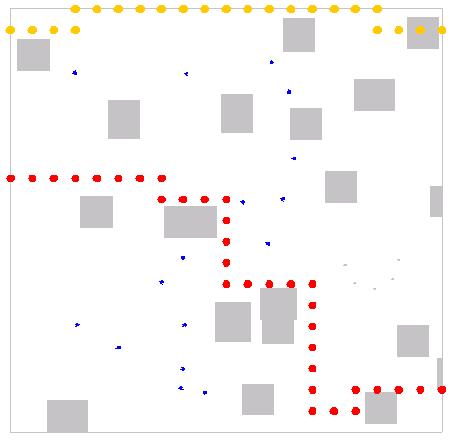
Figure 17.�
Autonomous deployment for barrier coverage with obstacles.
THIS PAGE INTENTIONALLY LEFT BLANK
The
simulation can be run as a Java application or a Java applet.� Once started,
the objects and the internal component structures are created.� Based on the
parameters specified in an XML initialization file, a default scenario starts.�
Scenarios run to completion or until the user interrupts with input.� Several
scenarios can be started by clicking on an appropriate button, and others can
be loaded from XML scenario files.� In most cases, starting a scenario also
causes parameters to be loaded from XML files as well.� When a scenario
provides active 2D or 3D output, the user has several options for modifying the
view, such as zooming in/out and choosing which objects in the environment are
visible.� The program consists of over 50 Java classes and several XML data
files.� The source files occupy approximately 700kB and consist of over 30,000
lines of code.
For random deployment,
we generate random locations in the terrain and assign the sensors there.
We estimated the
probability of traversal detection as a function of the number of sensors by
repeated experiments.� Each time the barrier coverage probability was
calculated and saved.� The saved probabilities are used to compute a
probability density function.� Figure 18 shows some results for 2, 10, 15, and
20 sensors for occluded and unoccluded measurements.� Occluded measurements
take the effects of obstacles into account, while unoccluded measurements do
not.�
Figure
18.�
Probability density function for the distribution of traversal detection
coverage measured for deployments of 2, 10, 15, and 20 sensors.
For 2 sensors, the
highest density is near zero for unoccluded sensor detections and even lower
for occluded.� For 10, 15, and 20 sensors, the peak coverages get progressively
higher, as expected.� This also shows that 20 sensors provide ample coverage
for traversal detection.�
Now consider Figure
19, which shows the coverage for deployments of 19 sensors.� Notice how the
density fluctuates around 1.2 percent density between 30 and 100 percent
coverage, varying no more than 1.0 percent.� Later we show the number of
sensors causing an even spread of density values to be the number of sensors
that results in minimum cost when deploying in steps.
Figure 19.�
Probability density function for 19 sensors.
Obtaining the
probability of reaching a specified level of coverage, or the confidence level,
is accomplished by randomly deploying sensors repeatedly and computing the
percent of time the deployment achieves the specified level.� Figure 20 shows a
graph of the confidence level reaching 80% coverage for 0 to 60 sensors.� The
confidence level increases with the number of sensors deployed.

Figure 20.�
Probability that coverage is above 80% for varying number of sensors.
When deploying sensors
randomly, such as when dropping from aircraft or launching from artillery, the
question is how many to deploy.� A simulation can deploy a set of sensors and
measure the coverage.� If the desired level of coverage is not reached, deploy
another set until the desired level of coverage is reached.� Obviously, if
there are more sensors available than is necessary to completely cover the
sensor field, deploying all sensors at once would be wasteful.� If there are
1,000 sensors and only 100 are required, then less than 1,000 should be
deployed.� We could deploy sensors one at a time, which would minimize the
number of sensors deployed; however, if each deployment includes a fixed cost,
this would be expensive.�
To find the optimum
number of sensors to deploy at a time we first assign a cost to deploy a set of
sensors (Cd) and a cost to each sensor (Cs).� Figures 21 through 24 are graphs
of how much it costs to deploy a set of sensors at a time to achieve the
specified coverage.�
Figure
21.�
Cost of achieving 80% coverage as a function of the number of sensors
with Cd = 0 and Cs = 1.

Figure
22.�
Cost of achieving 80% coverage as a function of the number of sensors
with Cd = 5 and Cs = 1.
Figure
23.�
Cost of achieving 80% coverage as a function of the number of sensors
with Cd = 10 and Cs = 1.
Figure 24.�
Cost of achieving 80% coverage as a function of the number of sensors
with Cd = 100 and Cs = 1.
The first figure shows
that if deployment is free then it is most cost-effective to deploy one sensor
at a time until achieving the desired coverage.� The last shows that if
deploying costs 100 times as much as each sensor then it is better to deploy
many sensors each step.� The other figures show that deploying approximately 23
sensors each step minimizes cost.� Cost is achieved at nearly the same number
of sensors for occluded and unoccluded sensor measurements so finding the
minimum for one should be sufficient in practice.
Note
that the local minimums of 23 for cost correspond to Figure 19, where coverage
fluctuates between 30 and 100 percent with 19 sensors.� [CLO02] developed an
analytical explanation for the correspondence between the local minimum and the
number of sensors with a flat probability density.� They used the following
equation to describe the expected cost 
where n is the number of sensors deployed each step for a
total of S steps, and 1-Fn(v) is the confidence of
obtaining coverage of amount v with n sensors.� As described in [CLO02],
when the probability density varies widely the weight associated with the first
term of the sum increases rapidly while the weights associated with the higher
number of sensors decrease.� The cost increases again after this local minimum
as the increase in n compensates for the decrease in weights.�
Figure 25 compares
barrier coverage for each of the placement algorithms in a 400m2
sensor field.� Occluded means that objects in the environment block the energy
from target to sensor.� Measurements were obtained for area coverage and
barrier coverage, occluded and not occluded, for each of the deployment
algorithms described in the previous chapter.�
The graphs in Figure
25 show the coverage differences between algorithms when obstacles present
barriers to traversal but not to sensing.� Our analysis shows that the Greedy
algorithm is the worst coverage algorithm; however, our GreedyPath algorithm
performed well.� Note Random placement performed fairly well, which is
significant because it will usually be cheap to deploy randomly.�
Autonomous deployment
performed well for unoccluded (Figure 25) and occluded (Figure 26)
measurements.� The sensor vehicles were able to deploy using only local
information and no central planning.� For scenarios where many sensors have no
internal map of the environment, limited communication capabilities, and
limited power, this will be essential.�

Figure 25.�
Deployment algorithm comparison, not occluded.
When the effect of
obstacles is taken into account, the graphs in Figure 26 show the choice of
algorithm can have a significant effect on coverage.� Greedy again performs the
worst.� The Genetic and Simulated Annealing algorithms perform the best by far,
achieving 100% barrier coverage with far fewer sensors than the other
algorithms.� Figure 27 gives a time comparison of the algorithms.� GreedyPath
performed quite well considering it is also one of the fastest of the
algorithms.� Random did not perform as well, but did perform adequately
considering it is the fastest.� Best1st and Greedy are the slowest.� Genetic
and Simulated Annealing are the slowest with few sensors, but with more sensors
find optimal solutions quickly.�

Figure 26.�
Deployment algorithm comparison, occluded.

Figure 27.�
Deployment algorithm time comparison.
This work developed a
simulation environment to enable varied testing of coverage and deployment
issues in a wide variety of sensor networks.� Many types of sensors exist and
with different characteristics (mobility, power, sensing ability, etc.).� The
energy measured by the sensors varies.� Sensors exist that detect sound, light,
movement, vibration, radiation, chemical substances, and so on.� The
environment may have varying occlusion characteristics as well as areas where
the desire to detect a target is higher.� Different coverage measurement
schemes, different data fusion schemes, and different deployment algorithms
will need to be tested.� The number of possible combinations that are testable
with the program implemented for this thesis is large.
As for
future work, the directed grid used to measure barrier coverage can have
different levels of granularity.� With higher granularity, there are more grid
squares and the coverage metric should be more accurate.� Future work should
examine the effect of granularity on accuracy and time.� [MEG00] describes the use of Voronoi diagrams
for computing coverage similar to our use of directed grids.� Future work could
compare and contrast Voronoi diagrams with directed grids.��
In
[PRO00] the authors present a vigilance model which allows birds to control the
area a flock occupies as well as their vigilance rate.� An optimal strategy is
found for the birds under a variety of conditions.� Performing the two
contradictory tasks presented, feeding and avoiding becoming food, is analogous
to two sensor tasks, sensing phenomena and conserving energy.� Future work
could examine the models presented in [PRO00] and extend the theories to
optimize the tradeoff between frequent sensing and power conservation, for
example.��
This
thesis describes a vector-force algorithm that accomplishes autonomous
deployments for area and barrier coverage.� An evolutionary strategy is
described for autonomous sweep coverage.� Future work could develop an
evolutionary strategy for autonomous deployment of sensor vehicles.� Furthermore,
the autonomous barrier coverage algorithm could be extended to move in a
particular direction, thereby accomplishing sweep coverage.
Future
enhancements can be made to the size and scope of the environment.� For
simplicity, this thesis focused on a limited number of homogenous sensors in a
fixed area.� The application supports testing for heterogeneous sensors, as
well as different sensing models.� Also, the area to be covered does not need
to remain static.� Sensors covering the flank side of a mobile force would need
to move with the force and continuously update their positions.�
The
size of the environment and the number of entities can be increased in a few
ways.� One approach would be to have a larger sensor field aggregate the
information of several smaller sensor fields for coverage and deployment.�
However, a limiting factor is that all the sensors run on one machine unlike in
the independence of the real world.� Future work could simulate separate
computational entities and network communication, which should enable the size
to increase greatly.
This thesis has
explored coverage and deployment issues for mobile and non-mobile sensors.� A
simulation of a multi-agent expeditionary sensor network was created to
formulate and test search, coverage, and deployment algorithms.� In the course of this research we evaluated cost and
performance of deploying multiple homogenous sensors with a wide variety of
constraints.� The comparison of several deployment algorithms showed significant
insights, and novel autonomous deployment schemes were presented.� The
application and algorithms developed enable future modeling and simulation
efforts.
While the components implemented in this thesis do not
target any existing framework, the
concepts are applicable to a wide range of sensor coverage and deployment
problems.� Many possible scenarios can be built, tested, and compared.� This
allows for extensive simulation of varied platforms to guide future acquisition
and minimize cost.� The design of the application allows for future
extensibility with minimal modification to existing code.� The algorithms
described can be implemented in any programming language or sensor network.
All
application source code, examples, and binary distribution are available at the
NPS SAVAGE archive or by request to:
Dr. Neil Rowe:� ncrowe@nps.navy.mil.
THIS PAGE
INTENTIONALLY LEFT BLANK
[AKY02]�������� Akyildiz, I.F., Su, W., Sankarasubramaniam,
Y., Cayirci, E., �Wireless sensor networks: a survey,� Computer Networks, 38,
393-422, 2002.
[AXE84]��������� Axelrod, R., The Evolution of
Cooperation, Basic Books, 1984.
[AXE97]��������� Axelrod, R., The Complexity of
Cooperation:� Agent-Based Models of Competition and Collaboration, Princeton University
Press, 1997.
[BAT02]��������� Batalin, M.A., �Spreading Out: A Local
Approach to Multi-Robot Coverage,� Proceedings of the 6th
International Symposium on Distributed Autonomous Robotics Systems, Fukuoka, JA, 2002.
[BAT03]��������� Batalin, M.A., �Efficient Exploration
Without Localization,� Computer Science Dept., USC, 2003.
[BER00]��������� Berg, M., Kreveld, M., Overmans, M., and
Schwarzkopf, O.� Computational Geometry: Algorithms and Applications, Springer-Verlag,
2000.
[BIG98] ��������� Bigus, J.P., and Bigus, J., Constructing
Intelligent Agents with Java�, John Wiley & Sons, Inc, 1998.
[BOR90]��������� Borenstein, J., Koren, Y., �Real-Time
Obstacle Avoidance for Fast Mobile Robots in Cluttered Environments,�
Proceedings of the 1990 IEEE International Conference on Robotics and
Automation, Cincinnati, OH, 572-577, 1990.
[BOR96]��������� Borenstein, J., Everett, H.R., Feng, L.,
Wehe, D., �Mobile Robot Positioning � Sensors and Techniques,� Journal of Robotic
Systems, Special Issue on Mobile Robots, Vol. 14, 231-249, 1996.
[BUC02]��������� Buckland, Mat, AI Techniques for Game
Programming, Premier Press, 2002.
�
[BUG00]��������� Bugajska, M.D., Schultz, A.C.,
�Co-Evolution of Form and Function in the Design of Autonomous Agents: Micro
Air Vehicle Project,� Navy Center for Applied Research in Artificial
Intelligence, 2000.
[BUL01]��������� Bulusu, N., Heidemann, J., Estrin, D.,
�Adaptive Beacon Placement,� UCLA, Los Angeles, CA, 2001.
[CHA01]�������� Chakrabarty, K., Iyengar, S.S., Qi, H.,
Cho, E., �Coding Theory Framework for Target Location in Distributed Sensor
Networks,� Dept. of Computer and Electrical Engineering, Duke University, 2000.
[CHA02]�������� Chakrabarty, K., Iyengar, S.S., Qi, H.,
Cho, E., �Grid coverage for surveillance and target location in distributed
sensor networks,� IEEE Transactions on Computers, vol. 51, 2002.
[CHO01]�������� Choset, H., �Coverage for robotics � A
survey of recent results,� Annals of Mathematics and Artificial Intelligence,
31, 113-126, 2001.
[CLI96]���������� Cliff, D., Miller, G.F., �Co-evolution of
pursuit and evasion II: Simulation Methods and Results,� From Animals to
Animats 4: Proceedings of the Fourth International Conference on Simulation of
Adaptive Behavior (SAB96), MIT Press Bradford Books, 1996.
�[CLO01]�������� Clouqueur, T., Ramanathan, P., Saluja,
K.K., Wang, K., �Value-Fusion Versus Decision-Fusion for Fault-Tolerance in
Collaborative Target Detection in Sensor Networks,� Fusion 2001 Conference,
2001.
[CLO02]��������� Clouqueur, T., Phipatanasuphorn, V.,
Ramanathan, P., Saluja, K.K., �Sensor Deployment Strategy for Target
Detection,� WSNA�02, Atlanta, GA, 2002.
[DHI02]���������� Dhillon, S.S., Chakrabarty, K., �A
Fault-Tolerant Approach to Sensor Deployment in Distributed Sensor Networks,�
Dept. of EE & CE, Duke University, Durham, NC, 2002.
[DHI02a]�������� Dhillon, S.S., Chakarabarty, K., �Sensor
Placement for Grid Coverage under Imprecise Detections,� Dept. of EE & CE, Duke University, Durham, NC, 2002.
[DIC02]���������� Dickie, Alistair, Modeling Robot
Swarms using Agent-Based Simulation, Master�s Thesis, Naval Postgraduate
School, Monterey, CA, June 2002.
[DMS03] ������� Defense Modeling
and Simulation Office (DMSO).� �Smart Sensor Web:� Experiment Demos Network
Centric Warfare,� https://www.dmso.mil/public/pao/stories/y_2002/m_04/7-1-8, May, 2003.
[EST99]���������� Estrin, D., Govindan, R., Heidemann, J.,
Kumar, S., �Next century challenges: scalable coordination in sensor
networks,� ACM MobiCom�99, 263-270, 1999.
[EST02]���������� Estrin, D., Culler, D., Pister, K.,
Sukhatme, G., �Connecting the Physical World with Pervasive Networks,�
Pervasive Computing, IEEE, 59-69, 2002.
[GAG92] ������� Gage, D.W.� �Command Control for Many-Robot
Systems,� Proceedings of AUVS-92, Huntsville, AL, 22-24 June 1992.
[GAG92a] ������ Gage, D.W. �Sensor Abstractions to Support
Many-Robot Systems,� RDT&E Division, Naval Command Control and Ocean Surveillance Center, 1992.
[GAG93] ������� Gage, D.W.
�Randomized search strategies with imperfect sensors,�� Proceedings of SPIE
Mobile Robots VIII, Boston, 9-10 September 1993, pp 270-279.
[GAG98] ������� Gage, D.W.
�Randomized Search Strategies,� http://www.spawar.navy.mil/robots/research/manyrobo/randomize.html,
June, 2003.
[GOL01]��������� Goldberg, D.,
Mataric, M.J., �Robust Behavior-Based Control for Distributed Multi-Robot
Collection Taks,� USC, Los Angeles, CA, 2001.
[GOR00]�������� Gordon, D.F.,
Spears, W.M., Sokolsky, O., Lee, I., �Distributed Spatial Control, Global Monitoring
and Steering of Mobile Agents,� AI Center, NRL, Wash., DC, 2000.
[GUP03]��������� Gupta, H., Das,
W.R., Gu, Q., �Connected Sensor Cover: Self-Organization of Sensor Networks for
Efficient Query Execution,� Mobihoc�03, Annapolis, MA, 2003.
[HES99]��������� Hespanha, J.P,
Kim, H.J., Sastry, S., �Multiple-Agent Probabilistic Pursuit-Evasion Games,�
Proceedings of the 38th Conference on Decision and Control, 1999.
[HOW01]������� Howard, A.,
Mataric, M.J., �Cover Me! A Self-Deployment Algorithm for Mobile Sensor
Networks,� Robotics Research Lab, USC, 2001.
[HOW02]������� Howard, A.,
Mataric, M.J., Sukhatme, G.S., �Mobile Sensor Network Deployment using
Potential Fields: A Distributed, Scalable Solution to the Area Coverage
Problem,� Proceedings of the 6th International Symposium on
Distributed Autonomous Robotics Systems (DARS02), Fukuoka, JA, 2002.�
[HOW02a]����� Howard, A.,
Mataric, M.J., Sukhatme, G.S., �An Incremental Deployment Algorithm for Mobile
Robot Teams,�� IEEE/RSJ International Conference on Intelligent Robots and
Systems (IROS2002), EPFL, SW, 2002.
[HOW02b]����� Howard, A.,
Mataric, M.J., Sukhatme, G.S., �An Incremental Self-Deployment Algorithm for
Mobile Sensor Networks,� �Autonomous Robots, Special Issue on Intelligent
Systems, 2002.
[HSI03]���������� Hsiang, T.,
Arkin, E.M., Bender, M.A., Fekete, S.P., Mitchell, J.S.B, �Algorithms for
Rapidly Dispersing Robot Swarms in Unknown Environments,� Stony Brook
University, NY, 2003.
[JUN02]��������� Jung, B.,
Sukhatme, G.S., �A Region-Based Approach for Cooperative Multi-Target Tracking
in a Structured Environment,� 2002 IEEE/RSJ International Conference on
Intelligent Robots and Systems, 2002.
[KOH00] ������� Kohout, B.
�Challenges in Real-Time Obstacle Avoidance,� Veridian/Pacific-Sierra Research,
Rosslyn, VA, 2000
[KOR91]�������� Koren, Y.,
Borenstein, J., �Potential Field Methods and Their Inherent Limitations for
Mobile Robot Navigation,� Proceedings of the IEEE Conference on Robotics and
Automation, 1398-1404, 1991.
[KIN91]��������� Kindl, M.R.,
Shing, M., Rowe, N.C., �A Stochastic Approach to the Weighted-Region Problem:�
Design and Testing of a Path Annealing Algorithm,� Naval Center for Applied
Research in Artificial Intelligence, 1991.
[LAV97]��������� LaValle, S.M.,
Lin, D., Guibas, L.J., Latombe, J., Motwani, R., �Finding an Unpredictable
Target in a Workspace with Obstacles,� Proceedings of the 1997 IEEE
International Conference on Robotics and Automation,1997.
[LUN01]��������� Lund, H.H,
Pagliarini, L., �Edutainment Robotics: Applying Modern AI Techniques,�
Proceedings of International Conference on Autonomous Minirobots for Research
and Edutainment (AMIRE-2001), 2001.
[MAR96]�������� Marengoni, M.,
Draper, B., Hanson, A., and Sitaraman, R.� �System to place observers on a
polyhedral terrain in polynomial time.�� Image and Visual Computing,
1996.
[MEG00]�������� Meguerdichian,
S., Koushanfar, F., Potkonjak, M., Srivastava, M.B., �Coverage Problems in
Wireless Ad-hoc Sensor Networks,� CS Dept and EE Dept, UCLA, 2000.
�
[MEG01]�������� Meguerdichian,
S., Koushanfar, F., Qu, G., Potkonjak, M., �Exposure in Wireless Ad-Hoc Sensor
Networks,� ACM SIGMOBILE, Rome, Italy, 2001.
[MIC00]��������� Michalewicz, Z.,
Fogel, D.B., How to Solve It: Modern Heuristics, Springer-Verlag Berlin
Heidelberg, NY, 2000.
[PAR00]��������� Park, S.,
Savvides, A., Srivastava, M.B., �SensorSim:� A Simulation Framework for Sensor
Networks,� EE Dept., UCLA, 2000.
[PAR98]��������� Parker, L.E.,
�Cooperative Robotics for Multi-Target Observation,� Center for Engineering
Systems Advanced Research (CESAR), Oak Ridge, TN, 1998.
[PER00]���������� Perkins, C. Ad
Hoc Networks, Addison-Wesley, 2000.
[PIS03] ���������� Pister, Kris.�
�Smart Dust.� Autonomous Sensing and Communicating in a Cubic Millimeter,� http://robotics.eecs.berkeley.edu/~pister//SmartDust/,
August, 2003.
[PRO00] �������� Proctor, C.J.,
Broom, M., �A Spatial Model of Anti-Predator Vigilance,� Centre for Statistics
and Stochastic Modeling, University of Sussex, 2000.
[REY99]��������� Reynolds, C.W.,
�Steering Behaviors for Autonomous Characters,� Sony Computer Entertainment
America, Foster City, CA, 1999.
[ROM02]�������� Romer, K.,
Kasten, O., Mattern, F., �Middleware Challenges for Wireless Sensor Networks,� Mobile
Computing and Communications Review, Vol. l6, 2, 2002.
[ROU98]�������� Roumeliotis,
S.I., Pirjanian, P., Mataric, M.J., �Ant-Inspired Navigation in Unknown Environments,�
Computer Science Dept, USC, 2002.
[RUS95]��������� Russell, S. and
Norvig, P.� Artificial Intelligence: A Modern Approach.��
Prentice-Hall, Inc,� 1999.
[SIN96]���������� Singh, S., Bertsekas, D. �Reinforcement
Learning for Dynamic Channel Allocation in Cellular Telephone Systems,� NIPS96,
Section: Applications, 1996.
[SIN01]���������� Singh, S.N.P., Thayer, S.M., �Immunology
Directed Methods for Distributed Robotics: A Novel, Immunity-Based Architecture
for Robust Control & Coordination,� Robotics Institute, CMU, 2001.
[SPE99]���������� Spears, W.M., Gordon, D.F., �Using
Artificial Physics to Control Agents,� AI Center, Naval Research Laboratory,
Washington, DC, 1999.
[STE95]���������� Stentz, A., �The Focussed D* Algorithm
for Real-Time Replanning,� Robotics Institute, CMU, 1995.
[STO96]��������� Stork, K.A., Sensors in Object Oriented
Discrete Event Simulation, Master�s Thesis, Naval Postgraduate School,
Monterey, CA, September 1996.
[TIL02] ���������� Tilak, S., Abu-Ghazaleh, N.B.,
Heinzelman, W., �A Taxonomy of Wireless Micro-Sensor Network Models,� Mobile
Computing and Communications Review, Vol. 1, Num. 2, 2002.
[ULR00]��������� Ulrich, I., Borentstein, J., �VFH*: Local
Obstacle Avoidance with Look-Ahead Verification,� 2000 IEEE International
Conference on Robotics and Automation, San Francisco, CA, 2505-2511, 2000.
[VAU94]�������� Vaughan, R., Sumpter, N., Henderson, J.,
Frost, A., Cameron, S., �Robot Control of Animal Flocks,� BioEngineering
Division, Silsoe Research Institute, Silsoe, Bedford, UK, 1995.
[WAT01]�������� Watt, A.,
Policarpo, F. 3D Games: Real-time Rendering and Software Technology,
Addison-Wesley, 2001.
[WEI99]��������� Weiss,
Gerhard. Multiagent Systems: A Modern Approach to Distributed Artificial
Intelligence. The MIT Press, 1999.
[ZOU03]��������� Zou, Y., Chakrabarty, K., �Sensor
Deployment and Target Localization Based on Virtual Forces,� Dept. of EE &
CE, Duke University, Durham, NC, 2003.
1.
Defense Technical Information Center
Ft. Belvoir, Virginia
2.
Dudley Knox Library
Naval Postgraduate School
Monterey, California
3.
Marine Corps Representative
Naval Postgraduate School
Monterey, California
4.
Director, Training and Education, MCCDC, Code C46
Quantico, Virginia
5.
Director, Marine Corps Research Center, MCCDC, Code C40RC
Quantico, Virginia
6.
Marine Corps Tactical Systems Support Activity (Attn:� Operations
Officer)
Camp Pendleton, California