To be replaced by your thesis processor using the data from your Python Thesis Dashboard

NAVAL POSTGRADUATE SCHOOL

MONTEREY, CALIFORNIA

THESIS

USING TEXTURE VECTOR ANALYSIS TO MEASURE COMPUTER AND DEVICE FILE SIMILARITY

by Bruce Allen

December 2019

Thesis Co-Advisors: Neil C. Rowe James Bret Michael

Approved for public release. Distribution is unlimited

THIS PAGE INTENTIONALLY LEFT BLANK

To be replaced by your thesis processor using the data from your Python Thesis Dashboard

NSN 7540-01-280-5500 Standard Form 298 (Rev. 2–89)

Prescribed by ANSI Std. 239–18

THIS PAGE INTENTIONALLY LEFT BLANK

To be replaced by your thesis processor using the data from your Python Thesis Dashboard

Approved for public release. Distribution is unlimited

USING TEXTURE VECTOR ANALYSIS TO MEASURE COMPUTER AND DEVICE FILE SIMILARITY

Bruce Allen Civilian

B.S., CSU Sacramento, 1989

Submitted in partial fulfillment of the requirements for the degree of

MASTER OF SCIENCE IN COMPUTER SCIENCE

from the

NAVAL POSTGRADUATE SCHOOL

December 2019

Approved by: Neil C. Rowe Thesis Co-Advisor

James Bret Michael Thesis Co-Advisor

Peter J. Denning

Chair, Department of Computer Science

THIS PAGE INTENTIONALLY LEFT BLANK

To be replaced by your thesis processor using the data from your Python Thesis Dashboard

ABSTRACT

Executable programs run on computers and digital devices. These programs are stored as executable files in storage media such as disk drives or solid state storage drives within the device, and are opened and run. Some executable files are pre-installed by the device vendor. Other executable files may be installed by downloading them from the Internet or by copying them in from an external storage media such as a memory stick or CD. It is useful to study file similarity between executable files to verify valid updates, identify potential copyright infringement, identify malware, and detect other abuse of purchased software. An alternative to relying on simplistic methods of file comparison, such as comparing their hash codes to see if they are identical, is to identify the “texture” of files and then assess its similarity between files. To test this idea, we experimented with a sample of 23 Windows executable file families and 1386 files. We identify points of similarity between files by comparing sections of data in their standard deviations, means, modes, mode counts, and entropies. When vectors are sufficiently similar, we calculate the offsets (shifts) between the sections to get them to align. Using a histogram, we find the most-likely offsets for blocks of similar code. Results of the experiments indicate that this approach can measure file similarity efficiently. By plotting similarity vs. time, we track the progression of similarity between files.

THIS PAGE INTENTIONALLY LEFT BLANK

Table of Contents

1. Introduction 1

2. Background 3

   1. Contents of an Executable File . . . . . . . . . . . . . . . . . . . 3

   2. Identifying File Similarity . . . . . . . . . . . . . . . . . . . . . 3

3. Calculating File Similarity 7

   1. Calculating Texture-Vector Data . . . . . . . . . . . . . . . . . . 7

   2. Calculating Similarity Offsets between Sections . . . . . . . . . . . . 9

   3. Calculating Similar-Section Offset Histograms. . . . . . . . . . . . . 10

   4. Calculating Similarity Measures Between Files . . . . . . . . . . . . 11

   5. Tracking Versions of Executable Code . . . . . . . . . . . . . . . . 13

4. Preparing the Dataset 15

   1. Preparing the Dataset of Executable Files. . . . . . . . . . . . . . . 15

   2. Preparing the Texture-Vector Files . . . . . . . . . . . . . . . . . 17

   3. Tuning Rejection Thresholds. . . . . . . . . . . . . . . . . . . . 19

   4. Preparing the Similarity-graph Files . . . . . . . . . . . . . . . . . 19

5. Results 21

   1. Evaluating Similarities by File Family . . . . . . . . . . . . . . . . 22

   2. Evaluating Similarities Across File Families. . . . . . . . . . . . . . 23

   3. Examining Similarity using the Texture-Vector Browser GUI Tool . . . . . 27

   4. Examining Similarity using Gephi . . . . . . . . . . . . . . . . . 34

6. Conclusions and Future Work 35

6.1 Conclusions . . . . . . . . . . . . . . . . . . . . . . . . . . 35

6.2 Future Work . . . . . . . . . . . . . . . . . . . . . . . . . . 35

Appendix A The Texture-Vector Similarity Toolset 37

A.1 Download . . . . . . . . . . . . . . . . . . . . . . . . . . . 37

A.2 Usage . . . . . . . . . . . . . . . . . . . . . . . . . . . . . 38

A.3 Texture-Vector Similarity Toolset Data . . . . . . . . . . . . . . . . 49

1. Texture-Vector Similarity Source Code . . . . . . . . . . . . . . . . 57

2. Source Code for Batch Processing. . . . . . . . . . . . . . . . . . 66

3. Source Code for Statistical Analysis . . . . . . . . . . . . . . . . . 67

E.4 Source Code License . . . . . . . . . . . . . . . . . . . . . . . 67

List of References 69

Initial Distribution List 71

List of Figures

Figure 4.1 Histogram of file sizes for our dataset. . . . . . . . . . . . . . . . 16

Figure 4.2 Histogram of file modification times for our dataset. . . . . . . . 17

Figure 5.1 Histogram of similarity matches across all files in our dataset. . . 21

Figure A.3 The TV file selection table. . . . . . . . . . . . . . . . . . . . . 45

Figure A.4 The similarity edge selection table for file node 10. . . . . . . . . 46

Figure A.5 The Texture-Vector Browser GUI showing file node 79 selected. . 48

List of Tables

THIS PAGE INTENTIONALLY LEFT BLANK

CHAPTER 1:‌

Introduction

Software of unknown pedigree abounds. This is partly due to software being distributed as executable code or a “binary”, and evaluating the contents of a binary is technically challenging.

Executable code consists of machine instructions, register references, memory addresses, hardcoded data, and text that is referenced by it. Machine instructions have operators and operands (arguments). When the source code changes with new versions and executable code is recompiled, most operands change. Small changes in source code can result in considerably different operands in the executables. Nonetheless, comparisons between versions of a binary can be made because most operators remain the same amongst the versions.

Machine instructions in executable code are interpreted by a processor. Programmers rarely write machine code directly. Instead, they write higher-level source code in a high-level language such as C++ and compile the source code into machine code.

Numerous updates to a binary can occur over the useful life of the executable to address new software requirements, fix software defects, or port the software to a different computing platform. Each of these requires recompilation and results in a new binary.

Executable code can be analyzed using reverse-engineering tools that recover information about the binary’s structure, function, and behavior. Some tools recognize data regions inside the code, while more advanced tools analyze the machine instructions to make inferences about the code’s function. Because of the differences in instruction set archi- tectures (ISAs), tools use models of ISAs. However, reverse engineering of a binary can be resource-intensive and can be stymied by deliberate anti-reversing techniques used to protect the binary file.

Executable code is vulnerable to malware. By replacing machine instructions with malicious ones, executable code can be transformed into malware. Malware can divert execution of code to perform one or more malicious tasks. Detection of malware contained in adversarial

malware binaries is technically challenging, even with the use of artificial-intellegence techniques such as deep learning [1].

We introduce here an approach based on texture vectors to allow executables to be compared against each other without requiring reverse engineering of the binaries. Our approach can be used as a first step to determine whether reverse engineering is needed. Chapter 2 covers related work. Chapter 3 describes the algorithms for creating texture vectors and processing them to draw conclusions about similarities between executable code files. Chapter 4 describes the dataset we used and how we prepared texture-vector and similarity-graph data. Texture-vector analysis using a dataset of executable files is presented in Chapter 5, followed by conclusions and recommendations for future work in Chapter 6. Details of the tools that implement the algorithms are presented in the appendices.

CHAPTER 2:‌

Background

1. Contents of an Executable File‌

   A binary contains more than just executable code. It includes fixed data, reserved space, and links to executable code that is external to the file [2]. Similarities in fixed data and fixed links are easiest to find because they can be matched directly. Reserved space usually consists of bytes with zero values, and is found in many places in a typical executable file. It can complicate similarity measurements since there can be many false matches with zero bytes.

   The portion of an executable file that contains the actual executable code consists of machine instructions and their associated operands. When executable code is modified, many machine instructions remain the same but usually their locations shift. Then the memory addresses encoded in their operands may change to compensate for this shift unless the code uses addressing relative to a register. However, register arguments encoded in operands may also shift. For 32-bit processors, many machine instructions are spaced four bytes apart; for 64-bit processors, eight bytes apart. Hence it may be possible to detect code similarity of machine instructions by comparing bytes at 4-byte or 8-byte boundaries.‌

   
   

2. Identifying File Similarity

   Numerous approaches exist for identifying similarities between files. They can be used on text files, binary files, images, video, and audio. A few apply to files containing executable code. Some of these executable-analysis tools visualize software evolution in source code using version-control information or source-code file analysis [3]. A three-dimensional graph can show where code accesses the operating system or other information about code flow, and graph how these numbers change over the evolution of a software product. The Code Time Machine tool [4] does this to show the evolution of code metrics for a given file. It shows values along a time-line for the number of lines of code, number of methods, and cyclomatic complexity (i.e., the number of paths the code can take given the possible

   
   

   conditions written into the code). A three-dimensional graph of files and file relations between versions relates files. Circles represent releases, squares represent files, and edges represent associations [5]. Other tools that graph code evolution are CVSScan [6] and EPOSee [7].

   There are many types of files. Three important ones are:

   • Text: Text typically consists of words arranged in sentences. It may also be frag- mented because of formatting, as in a formatted PDF file, or may be in short phrases in data tables or in the data section of executable code. We can measure text similarity by comparing words.

   • Arbitrary bytes: What may appear as arbitrary bytes may be numeric data, com- pressed data, or executable codes. Numeric data often has low entropy because many of the bytes tend to be zero. Compressed data has high entropy because unused byte patterns in the data are removed.

   • Audio and video: Audio and video data consists of bytes arranged in sequences. Bytes can be compared by aligning the sequences.

     There are many algorithms for identifying similarities in data. Some work better than others given the type of data being compared. Methods used in comparing files are:

   • Comparing byte sequences: Comparing content of text files to identify similarity is a common operation. One approach tries to find the longest common subsequences [8], where text that does not match is identified as new or deleted content. Algorithms for efficient string matching include Knuth-Morris-Pratt [9], which allows searching without backtracking when a near match is found and Boyer-Moore [10], which skips alignments when searching for specific text. Although intended for text, both algorithms may be used with executable code. Another popular algorithm for text files is implemented in the “diff” utility developed for the Linux operating system [11]. It compares lines delineated by carriage returns in one file against those in another file by concurrently passing through both files. However, when identical lines are at different locations in two files, diff can return false positives or negatives. Given that diff exploits carriage returns which are not common in executable code, and that executable code may be moved around by the compiler, diff is unsuitable for matching files of executable code.

     
     

   • Comparing executable bytes: Comparing bytes in files is similar to comparing text in files. However, bytes of files containing executable code are unlikely to match on operands and thus only the operators should be compared. For Intel architectures, operands are usually spaced at 4-byte or 8-byte intervals. Because of this, [12] says that “binary file analysis by both binary diffing and cryptographic hash signatures comparison is a very limited approach to identify source code being re-used” and suggests metadata analysis. Regardless, for Intel architectures, it is useful to compare at every fourth or eighth byte because this will often align runs of comparisons with operators.

   • Comparing histograms: We can identify common sequences of N bytes (“N-grams”) between files, contiguous sequences of bytes of a given length and compute a his- togram of them. In [13], 5-grams are used, and a Bloom filter is used as an efficient data structure for storing N-gram patterns that are found. Overall file similarity can be measured with the Jaccard index, the count of N-grams in common divided by number of distinct N-grams in both files. To take frequencies of the N-grams into account in measuring similarity, the cosine similarity or the Kullback-Leibler divergence can be used [14].

   • Transforming values before comparison: It may work better to measure similarity on transforms of the data values. This is commonly done for audio and video data; perceptual hashing [15] provides a similar hash output if features are similar. For images, we can transform the image to frequency space, or apply convolutions to it to enhance features. For signals, we can apply the Fourier transform to obtain frequencies.

   • Comparing metadata: Initial comparisons of files can use their descriptive data to decide if they are sufficiently related to be worth further analysis. For example, if we know two executable files are built to run on a Microsoft Windows system using the same Intel instruction-set architecture, they are worth comparing. We can also compare metadata about sections and data structures within the files [12]. Metadata includes:

     • File types and subtypes.

     • Data compression parameters. Cloning is indicated if the compressed size is significantly smaller than the combined size of its parts [12].

     • Mentions of precompiled libraries.

       
       

     • Hashcodes on the files.

   • Comparing decompiled data: Executable files can be decompiled into text, and we can compare this text. Disassemblers and decompilers can do this, though they are not perfect. Disassemblers turn the bytes of executable code into corresponding machine code mnemonics and symbolic names, addresses, and offsets. Decompilers go further by turning bytes into source code.

     Identifying similarity specifically between versions of source code can be accomplished in several ways:

   • Object-oriented analysis: Software objects in source-code versions can be visually compared using a difference graph [16]. A graph of each version can be created where nodes are classes and node attributes are class methods and variables. Edges connect nodes where attributes of one node reference attributes of another. Then a class relation diagram is constructed that highlights differences in class relations in two software versions.

   • Software-diagram analysis: Software diagrams created during design may be com- pared if available [17].

   • Version control analysis: Many products used by the software industry manage source code versioning with a repository [18]. Then there is often documentation of the differences between versions.

CHAPTER 3:‌

Calculating File Similarity

In this chapter we present our texture-vector approach. We perform three layers of calcu- lations to make inferences about similarity and how and where files are similar. Our steps are:

1. Calculate texture-vector datasets from the two files to be compared.

2. Compare texture-vector datasets to identify similarity offsets and produce a similarity offset histogram.

3. Calculate statistics from the heights of the similarity offset histogram to produce a single similarity measure for the comparison of the two files.

This process is illustrated in Figure 3.1.

Figure 3.1. Inference process.

1. Calculating Texture-Vector Data‌

   Texture vectors are calculated from the byte values of contiguous sections of binary data. Although many transform algorithms are possible, we are specifically interested in trans- forms that can both represent some unique characteristic of the data and possess a value that can be meaningfully compared to other values to measure similarity.

   Sections measured as similar by many transforms have stronger similarities than others. We tested the following transforms for calculating texture vectors on the integer values of the bytes:

   • Standard Deviation: The standard deviation of the byte values in a section of binary data. Two sections with a similar amount of deviation may be similar.

     
     

   • Mean: The average byte value in the section. When executable code changes, operators may remain the same and help maintain the same mean.

   • Mode: The most frequent byte value in the section. Often this value was zero in our data. This value is nonmetric and can only be used in computing similarity distances in the sense that it is identical or not.

   • Mode Count: The count of occurrence of the most frequent byte value in the section.

   • Entropy: The Shannon entropy of the byte values in the section. Two sections may be similar if the amount of randomness in each section is similar.

We considered a Fourier transform for texture values, but chose not to because it preserves information and returns output the same size as the input. We could have used lowpass or highpass filtering to reduce the number of values it found, but found that similar data was provided by the entropy measure.

We picked a section size of 500 for the texture vectors after experimenting with low values such as 50 and high values such as 50,000. A section size that was too small resulted in texture vectors with too much fluctuation, and a section size that was too large diluted the texture-vector characteristics. We also picked 500 rather than a size that is the power of two so as to not attempt to align with possible data structure sizes or boundaries intrinsic to specific data such as organizational boundaries of contents placed within executable code.

3.1.1 Calculating Texture-Vector Distance

Two texture vectors are defined as similar when the first texture-vector is within a threshold of closeness to the second texture vector by the weighted square of the L2 (Euclidean) distance metric [19]. The similarity can be thought of as 1/d2 where d is distance, calculated as: d = w1(dv1)2 + w2(dv2)2 + w3(dv3)2 + w4(dv4)2 + w5(dv5)2 where dv is the difference at a given vector element and w is the weight for a given vector element. For example if texture-vector 1 has values [100, 30, 220, 50, 80], texture-vector 2 has values [101, 32,225,

51, 80], and weights [w1, w2, w3, w4, w5] are [0.25, 0.25, 0.0, 0.25, 0.25], then the L2 distance

d2 is 0.25 ∗ 12 + 0.25 ∗ 22 + 0.0 ∗ 52 + 0.25 ∗ 12 + 0.25 ∗ 02 = 0.25 + 1.0 + 0 + 0.25 + 0 = 1.5.

A threshold of similarity was used for our graphics; for instance, if the acceptance threshold is 1.0, these vectors are not similar because 1.5 i 1.0. We set weight values by experiment as explained in Chapter 4.3. A good threshold identifies numerous correct similarities

between the sections of data from which the texture vectors were calculated while excluding non-similarities.

In our experiments, we saw many byte ranges of very low entropy, for example where all but three byte values in a section were 0. If low-entropy occurrences are random, then they average out somewhat in the mean power histogram described in Chapter 3.3. If they are not random, they can still be useful in identifying similarity. We decided not remove any texture vectors such as those with extremely low entropy because we want our similarity algorithms to use all the data. However, future work should consider weighting bytes by their inverse document frequency, traditionally computed as the inverse of the logarithm of their count.‌

1. Calculating Similarity Offsets between Sections

   We calculate similarity offsets by comparing all the texture vectors in one file against all the texture vectors in another file and counting the offsets between the files where the texture vector distance is within the threshold of closeness. When there are many offsets with the same value, this gives high confidence in those byte matches.

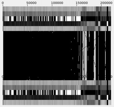
   We implemented a display to show consistently strong offsets between two files. The display draws lines connecting similar texture vectors. The pattern and quantity of similarity lines indicates the nature and degree of file similarity. Figure 3.2 shows an example of two very similar versions of executable code, where the texture vector pattern of each file is shown across the top and bottom, and the lines between them indicate points of similarity. The files are both roughly 220 KB in length.

   
   

   

   Figure 3.2. Texture patterns of two very similar executable files and lines connecting them indicating points of similarity.

   
   

2. Calculating Similar-Section Offset Histograms‌

   We calculate a similarity offset histogram from the set of offsets identified when searching for sufficiently similar texture vectors. There can be many thousands of offset values where similar-section matches can occur. To quantify this distribution of offsets, we create a similarity offset histogram and distribute calculated offset values across approximately 400 buckets, which sufficiently categorizes offsets in a viewable form. Consistent offset values are found as peaks on the histogram of offset values and represent likely meaningful similarities.

   We calculate the measure of similarity between two files from the heights in the similarity offset histogram to provide a numeric measure of similarity between files. A large spread in heights suggests similarity at specific offsets, indicating similarity, while minimal spread in heights suggests a random distribution of similarity offsets, likely a result of false positives.

   Because it is mathematically possible to have more similarity offsets near the middle of the

   
   

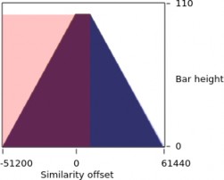
   histogram than at the sides, we must adjust histogram counts by offset value. We created a compensated histogram that has an even probability of heights across it, and calculated similarity from that. We calculated the compensated histogram by removing the right side of the histogram where the possibility for histogram counts is decreasing, and added it to the left side, where the possibility for histogram counts is increasing. This is shown in Figure 3.3, where the triangular region is the uncompensated histogram and the rectangular region is compensated. The horizontal axis plots the number of similarity offsets found for each bucket. The offset value along the horizontal axis is the difference between the byte location of the similar-section offset in one file and the byte location of the matching similar-section offset in the other. The horizontal axis spans from the negative of the size of the file on the left to the positive size of the file on the right. Although the ordering of the files are user-selected, the calculated histogram is identical; the calculation is symmetric. Because these histograms overlap on the graph, we draw them slightly transparent so they blend, allowing us to see all their parts.

   
   

   

   Figure 3.3. An illustration showing an uncompensated histogram (triangular region) and its equivalent compensated histogram (rectangular regin) used for the similarity calculation.

   
   

3. Calculating Similarity Measures Between Files‌

   We calculate the measure of similarity between two files from the magnitude of the standard deviation of the heights of the compensated histogram as described in Chapter 3.3. An example of calculated similarity measure, along with the texture vectors, similarity offsets, and similar-section offset histograms, is shown in Figure 3.4. The top part describes the files

   
   

   being compared, the weights used in calculating the texture-vector distance, and statistics about the view, including the calculated similarity measure of 334.3535. The middle part shows the two texture-vector patterns, which visually appear identical, along with the center region saturated black with similarity lines. The bottom part shows the similarity histograms, where the similar-section offset histograms have spikes and low points. We will conclude that these two files are nearly identical in Chapter 5.

   
   

   

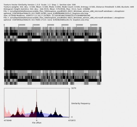
   Figure 3.4. Example of high value of high similarity in file family

   iexplore_exe.

   
   

4. Tracking Versions of Executable Code‌

We can also graph a network of relationships between different versions of the same ex- ecutable. By using the file modification time for the horizontal axis and the calculated similarity measure described in Chapter 3.4 as the vertical axis, we can show the relation- ships between versions. Files that have a larger similarity measure to the selected file are plotted higher on the vertical axis. Files whose similarity measure is below a user-selectable measure are not plotted. By adjusting the similarity threshold using the SD slider described in Appendix A.2.4, we can remove files with minimal similarity to reveal clusters of files that match with greater similarity. Using this graph, we can make inferences; for example, releases with a similar modification time may be a result of bug fixes or security updates; releases with a smaller similarity measure may have more functional differences or may have added malware. An example of this graph is shown in Figure 5.6.

THIS PAGE INTENTIONALLY LEFT BLANK

CHAPTER 4:‌

Preparing the Dataset

The dataset we studied consisted of executable files, texture-vector files, and similarity-graph files.‌

4.1 Preparing the Dataset of Executable Files

The initial set of files was a sample of executable .exe and .dll files extracted from the Real Data Corpus [20]. The Real Data Corpus consists of “images” (copies) of used disk drives and other devices obtained from non-U.S. countries. The files were extracted using the icat extraction tool from The Sleuth Kit forensics tool, https://forensicswiki.org/wiki/ The_Sleuth_Kit. Prof. Rowe picked 23 representative families of executables defined by a file name for each. Since many of the files were faulty, he used a software wrapper that loaded files for each distinct file contents (as indicated by its hash code) until the wrapper found a non-faulty copy. Names were changed from the original ones to distinguish files with the same names and different contents. The initial set consisted of 1,386 files. Of these, 162 were excluded because their size was greater than 1 MB and 55 were excluded because their size was less than 1 KB. Of the remaining 1,169 files, 35 were excluded because they were identical based on their MD5 cryptographic hash, leaving 1,134 files in our dataset. Figure 4.1 shows the distribution of file sizes. Note that since all files are from various countries and no files are from the U.S., our collection may exclude important versions of software.

Number of files by file size

250

Number of files

200

150

100

50

0

104 105 106

File size in bytes

Figure 4.1. Histogram of file sizes for our dataset.

The file modification times were extracted by Prof. Rowe using a separate pro- gram find_mod_times.py that uses DFXML metadata for the files created using the fiwalk program, https://www.forensicswiki.org/wiki/Fiwalk. We wrote a program set_modtimes.py (seeAppendix E.2.3), to set the file timestamps of these files using the MD5 cryptographic hash and timestamp information. We set these timestamps so that the file timestamp information can be captured as metadata when creating texture-vector datasets. The earliest valid modification timestamp value was used for each hashcode. Timestamps before 1979 were considered invalid. The distribution of files by file modification time is shown in Figure 4.2.

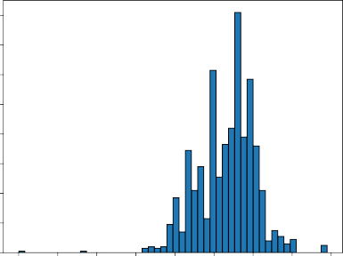
Number of files by modification time

160

140

Number of files

120

100

80

60

40

20

0

1980 1985 1990 1995 2000 2005 2010 2015 2020

Modification time

Figure 4.2. Histogram of file modification times for our dataset.

Statistics on the 23 file families that we studied are shown in Table 4.1. This includes source- code family tabulate_drive_data_py, which allows us to compare some versioned source-code files too.

Filenames for executable files in our dataset were assigned by Prof. Rowe to have a country- of-origin prefix followed by a drive code, followed by the absolute path to the file within the drive, followed by the filename, and finally followed by the .tmp suffix. All slashes and spaces are replaced with underscores for convenient storage in a Linux file system. A .tmp suffix is appended so that the file manager does not display them as executable files.‌

1. Preparing the Texture-Vector Files

   We created the texture-vector .tv files with the sbatch_calc_tv.bash program described in Appendix E.2. Due to the computational burden, we calculated texture vectors on the Naval Postgraduate School (NPS) Hamming supercomputer using sbatch parallel processing. Sbatch is a Slurm workload manager that schedules jobs across multiple

   
   

   Table 4.1. Files by file family.

   

   
   

   File Family	File count	Min file size	Max file size	Mean file size	Standard deviation of file size
   a0003775_dll	14	1591	853504	258271.6	318135.5
   bthserv_dll	37	1067	92160	31455.4	19509.8
   ccalert_dll	23	189560	267880	225524.2	21199.8
   cdfview_dll	244	1178	409600	144513.2	39662.1
   dunzip32_dll	34	11091	149040	114370.9	26991.3
   hotfix_exe	33	53248	112912	94098.4	13263.9
   iexplore_exe	216	3506	903168	461304.5	277712.7
   mobsync_exe	80	8192	970752	156818.5	141438.6
   msrdc_dll	6	159232	194048	174933.3	15696.5
   nvrshu_dll	32	151552	262144	240128.0	33724.4
   pacman_exe	2	165594	241693	203643.5	53810.1
   policytool_exe	104	1224	787508	54764.8	84605.1
   powerpnt_exe	19	2310	676112	366290.8	236454.6
   rtinstaller32_exe	4	135168	158312	146740.0	9843.3
   safrslv_dll	29	1582	65536	41681.3	12648.2
   tabulate_drive_data_py	23	18647	47544	34090.3	7213.7
   typeaheadfind_dll	2	35920	39856	37888.0	2783.2
   udlaunch_exe	4	118784	118784	118784.0	0.0
   vsplugin_dll	8	65606	118801	88180.2	15049.3
   webclnt_dll	80	1261	611328	96930.6	92513.1
   winprint_dll	7	12048	44544	29627.4	13120.4
   wmplayer_exe	120	2864	520192	142871.3	101072.6
   xrxwiadr_dll	13	8192	311296	123327.4	75040.4

   
   

   processors (see https://slurm.schedmd.com/overview.html). This program runs one job per file. Jobs take varying times to complete because file sizes vary. To compute the texture vectors for the 1,134 jobs, with a job queue size of 500, took about two minutes.

   We then copied these .tv files to the Texture-Vector Similarity repository, renaming them to their MD5 cryptographic hash value, for access by the Texture-Vector Similarity GUI tool, by running md5copy_500.py, see Appendix E.2.3.

   
   

2. Tuning Rejection Thresholds‌

Similarity is indicated when the square of the L2 distance measure is less than an acceptance threshold, as described in Chapter 3.1.1. We performed our tuning with two arbitrarily selected larger files in the ccalert_dll file family. We began with a default weight of

0.5 for the standard deviation, mean, mode count, and entropy transforms and, after some experimentation, we selected a distance rejection threshold of 5.0 because it resulted in reasonable similarity offsets without an oversaturation of matches. We selected a default weight of 0.0 for the mode because mode values do not quantifiably compare with each other, though an alternative could be to set distances between modes to 0 for identical values and 1 for nonidentical values.

We examined our tuning of weight values by setting all weight values to 0.0 and then, one weight at a time, examined the saturation of matched offsets as we adjusted the weight for each texture contribution from 0.0 to 1.0. For each weight adjustment, we observed that the quantity of similarity offsets identified would vary as we changed the weight and also that there was a visually understandable quantity of similarity at weight 0.5. Given this, we accepted our weight and rejection threshold values as our default values. These defaults are shown in Table 4.2.

Table 4.2. Default texture-vector threshold settings.

4.4 Preparing the Similarity-graph Files‌

We created the similarity-graph files by running the sbatch_ddiff_tv.bash program as described in Appendix E.2. We calculated the similarity metrics on the NPS Hamming supercomputer using sbatch parallel processing with a job queue size of 700, resulting in a graph of 1,134 nodes and 463,486 edges from which we can create a similarity matrix across all file families. We compared files across file families in order to measure similarity

between known dissimilar files. There are 642,411 possible edges, but we dropped 178,925 of them because they had less than two similarity matches. This processing took about fifteen hours. Runtime of each file pair varied because file sizes varied.

Node data consists of the node index, filename, file family, file size, file-modification time, and file MD5 hashcode, as described in Appendix A.2.4. Edge data consists of the edge’s source and target file node indexes along with the standard deviation, mean, maximum, and sum similarity metrics described in Chapter 3.4.

CHAPTER 5:‌

Results

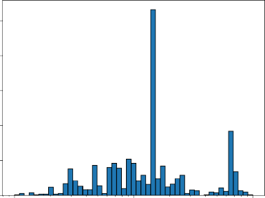
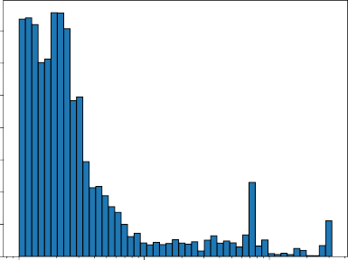
To evaluate the ability of our tools to identify similarities between executable files, we examined the 642,411 texture-vector similarity measures calculated for each pair of files for the 1,134 files. Of the 642,411 possible comparisons, 463,486 of them produced nonzero similarity values. Similarity measure values varied from zero to about 300. The distribution of these 463,486 similarity values across all files in our dataset is shown in Figure 5.1. Due to the uneven distribution of these values, a similarity threshold cannot be calculated using a normal gausian distribution. Most similarity measure values were less than ten, which is where the curve becomes level. This suggests that actual similarity between two files may be indicated when their similarity measure is greater than ten.

17500

Number of similarity matches

15000

12500

10000

7500

5000

2500

0

File similarity across all files

100 101 102

Similarity measure

Figure 5.1. Histogram of similarity matches across all files in our dataset.

1. Evaluating Similarities by File Family‌

   To establish a baseline of what the similarity measure values are for similar files, we calculated the mean similarity measures for files within file families, see Table 5.1. The number of comparisons made within each file family is also shown. These values establish similarity measures within individual file families, which establishes similarity values given ground truth.

   
   

   Table 5.1. Mean similarity and number of comparisons made within file families.

   
   

   File Family	Mean similarity	Number of compar- isons made for this file family
   a0003775_dll	4.5	72
   bthserv_dll	3.7	478
   ccalert_dll	11.4	253
   cdfview_dll	10.0	1487
   dunzip32_dll	5.1	554
   hotfix_exe	8.5	115
   iexplore_exe	130.2	22311
   mobsync_exe	6.1	1808
   msrdc_dll	4.5	15
   nvrshu_dll	32.9	496
   pacman_exe	1.5	1
   policytool_exe	2.6	223
   powerpnt_exe	76.0	125
   rtinstaller32_exe	13.4	6
   safrslv_dll	3.3	18
   tabulate_drive_data_py	2.8	253
   typeaheadfind_dll	2.3	1
   vsplugin_dll	3.2	24
   webclnt_dll	3.8	2247
   winprint_dll	1.1	21
   wmplayer_exe	9.1	6742
   xrxwiadr_dll	15.9	66

   
   

2. Evaluating Similarities Across File Families‌

   We tested whether the similarity measure between files of the same file family was higher than the similarity measure between files in different file families. The confusion matrix for file similarity across all file families in our dataset is in Table 5.2. Rows and columns represent file families using the numbers in the second column. The mean similarity measures between files within file families is typically greater than the mean similarity between files in other file families, showing that our approach for identifying file similarity is useful. We also compare similarity using texture-vectors vs. similarity using Prof. Rowe’s byte analysis which identifies file similarity by comparing similarity between byte values at two, four, and eight byte intervals. This is shown in Figure 5.2. Here we see a trend upward and to the right, indicating that both approaches agree in measuring similarity.

   
   

   

   
   

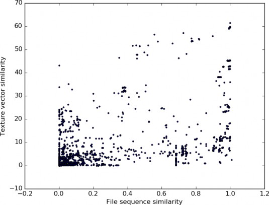
   Figure 5.2. Similarity using texture-vectors vs. similarity using Prof. Rowe’s byte analysis.

   
   

   Table 5.2. Mean file similarity between file families.

   

   
   

   Family	No.	1	2	3	4	5	6	7	8	9	10	11	12
   a0003775_dll	1	4.5	1.2	5.4	2.1	3.8	3.0	3.6	2.8	2.2	3.3	5.1	2.3
   bthserv_dll	2	1.2	3.7	1.2	0.7	0.7	0.7	0.5	0.7	0.6	0.3	0.9	0.6
   ccalert_dll	3	5.4	1.2	11.4	2.5	3.9	3.2	2.2	2.9	3.6	4.3	4.8	2.2
   cdfview_dll	4	2.1	0.7	2.5	10.0	1.3	1.1	1.6	2.2	1.8	0.9	1.7	0.8
   dunzip32_dll	5	3.8	0.7	3.9	1.3	5.1	2.3	4.0	2.1	2.0	3.4	3.6	1.6
   hotfix_exe	6	3.0	0.7	3.2	1.1	2.3	8.5	1.3	2.0	1.4	3.8	3.1	1.6
   iexplore_exe	7	3.6	0.5	2.2	1.6	4.0	1.3	130.2	9.3	1.6	2.4	1.5	7.5
   mobsync_exe	8	2.8	0.7	2.9	2.2	2.1	2.0	9.3	6.1	1.5	2.3	2.7	1.6
   msrdc_dll	9	2.2	0.6	3.6	1.8	2.0	1.4	1.6	1.5	4.5	1.4	2.0	0.9
   nvrshu_dll	10	3.3	0.3	4.3	0.9	3.4	3.8	2.4	2.3	1.4	32.9	6.2	2.1
   pacman_exe	11	5.1	0.9	4.8	1.7	3.6	3.1	1.5	2.7	2.0	6.2	1.5	2.2
   policytool_exe	12	2.3	0.6	2.2	0.8	1.6	1.6	7.5	1.6	0.9	2.1	2.2	2.6
   powerpnt_exe	13	3.5	0.4	2.2	1.1	3.1	1.5	41.2	5.8	1.4	2.6	2.2	4.6
   rtinstaller32_exe	14	3.4	0.9	4.1	2.0	3.6	2.0	1.6	2.3	2.2	2.3	2.8	1.2
   safrslv_dll	15	1.9	0.9	2.2	1.1	1.2	1.6	1.1	1.1	0.7	2.0	2.0	1.0
   tabulate_drive_data_py	16	0.1	0.1	0.1	0.1	0.1	0.1	0.2	0.1	-	0.1	-	0.3
   typeaheadfind_dll	17	0.9	0.6	1.3	0.7	0.4	0.3	0.4	0.5	0.7	0.1	0.7	0.5
   udlaunch_exe	18	2.9	0.4	3.3	1.1	2.5	-	1.3	1.7	1.8	3.3	3.0	-
   vsplugin_dll	19	3.0	0.6	3.4	1.0	2.0	2.5	4.0	1.8	1.2	3.2	3.0	1.6
   webclnt_dll	20	3.3	1.0	3.6	1.1	2.3	1.3	1.8	1.8	1.5	2.2	2.8	1.0
   winprint_dll	21	0.8	0.5	0.9	0.4	0.6	0.5	0.4	0.5	0.5	0.4	0.6	0.6
   wmplayer_exe	22	3.1	0.4	3.1	0.9	2.4	2.0	21.7	3.6	1.3	3.0	2.8	2.4
   xrxwiadr_dll	23	11.5	0.8	12.1	2.5	9.2	4.1	3.2	4.6	3.3	12.9	13.0	3.8

   
   

   Family	No.	13	14	15	16	17	18	19	20	21	22	23
   a0003775_dll	1	3.5	3.4	1.9	0.1	0.9	2.9	3.0	3.3	0.8	3.1	11.5
   bthserv_dll	2	0.4	0.9	0.9	0.1	0.6	0.4	0.6	1.0	0.5	0.4	0.8
   ccalert_dll	3	2.2	4.1	2.2	0.1	1.3	3.3	3.4	3.6	0.9	3.1	12.1
   cdfview_dll	4	1.1	2.0	1.1	0.1	0.7	1.1	1.0	1.1	0.4	0.9	2.5
   dunzip32_dll	5	3.1	3.6	1.2	0.1	0.4	2.5	2.0	2.3	0.6	2.4	9.2
   hotfix_exe	6	1.5	2.0	1.6	0.1	0.3	-	2.5	1.3	0.5	2.0	4.1
   iexplore_exe	7	41.2	1.6	1.1	0.2	0.4	1.3	4.0	1.8	0.4	21.7	3.2
   mobsync_exe	8	5.8	2.3	1.1	0.1	0.5	1.7	1.8	1.8	0.5	3.6	4.6
   msrdc_dll	9	1.4	2.2	0.7	-	0.7	1.8	1.2	1.5	0.5	1.3	3.3
   nvrshu_dll	10	2.6	2.3	2.0	0.1	0.1	3.3	3.2	2.2	0.4	3.0	12.9
   pacman_exe	11	2.2	2.8	2.0	-	0.7	3.0	3.0	2.8	0.6	2.8	13.0
   policytool_exe	12	4.6	1.2	1.0	0.3	0.5	-	1.6	1.0	0.6	2.4	3.8
   powerpnt_exe	13	76.0	1.5	1.0	0.2	0.2	1.5	2.8	1.7	0.3	12.6	8.2
   rtinstaller32_exe	14	1.5	13.4	1.1	0.1	0.4	3.1	1.9	2.0	0.6	1.7	6.3
   safrslv_dll	15	1.0	1.1	3.3	0.1	0.8	-	1.4	1.2	0.6	1.1	2.6
   tabulate_drive_data_py	16	0.2	0.1	0.1	2.8	0.1	-	0.2	0.2	-	0.1	0.3
   typeaheadfind_dll	17	0.2	0.4	0.8	0.1	2.3	0.2	0.5	0.8	0.4	0.2	0.6
   udlaunch_exe	18	1.5	3.1	-	-	0.2	-	2.1	0.9	0.5	2.2	3.6
   vsplugin_dll	19	2.8	1.9	1.4	0.2	0.5	2.1	3.2	1.7	0.5	2.7	3.5
   webclnt_dll	20	1.7	2.0	1.2	0.2	0.8	0.9	1.7	3.8	0.7	1.5	5.0
   winprint_dll	21	0.3	0.6	0.6	-	0.4	0.5	0.5	0.7	1.1	0.4	0.6
   wmplayer_exe	22	12.6	1.7	1.1	0.1	0.2	2.2	2.7	1.5	0.4	9.1	5.7
   xrxwiadr_dll	23	8.2	6.3	2.6	0.3	0.6	3.6	3.5	5.0	0.6	5.7	15.9

   
   

   Although the greatest average similarity for a given file family is usually within that file family, there are exceptions as between file families a0003775_dll and xrxwiadr_dll. This inconsistency could be due to the differences in file size or to other attributes within the files in these two file groups. An example similarity analysis plot illustrating the problem is Figure 5.3. Ranges of homogeneous texture vectors contain similar low mode counts

   
   

   and moderately high entropy values, suggesting that our similarity measure is primarily attributed to regions of compressed data rather than similarity in code. The few similarity matches in other regions suggest that there is actually little similarity between these two files.

   
   

   

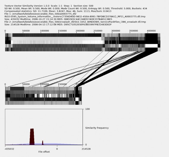
   Figure 5.3. False-positive similarity between two files caused by homoge- neous compressed data.

   
   

   As seen in Table 5.1, the mean similarity between files within file family varies greatly based on file family. For example mean similarity within the iexplore_exe family is

   130.2. An example comparison of two very similar files was shown in Figure 3.4, where

   
   

   the histogram shows regions of low similarity and regions of high similarity, resulting in the high calculated similarity value. Mean similarity within the winprint_dll file family is 1.1. An example comparison of two files within this family is shown in Figure 5.4. The histogram shows a fairly even dispersion of similarity, with no offset in particular matching mor than other offsets.

   
   

   

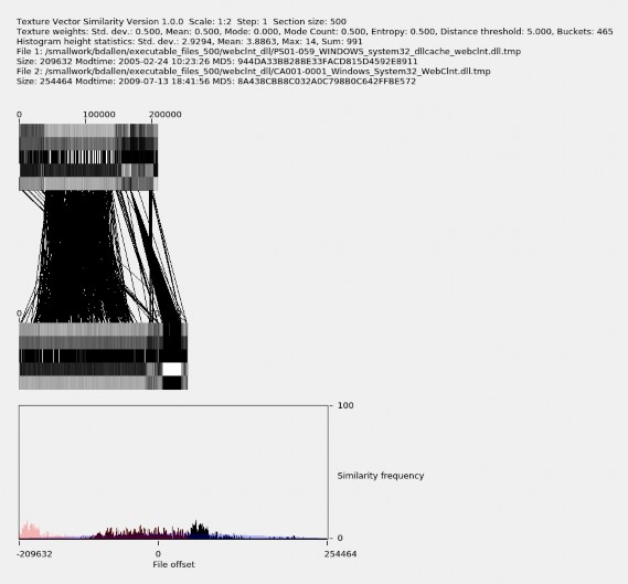
   Figure 5.4. Example of low value of high similarity in file family

   winprint_dll.

   
   

   Average similarity measures between files across file families also varies greatly, as shown in Table 5.2. Average similarity between files of different file families tend to be high when

   
   

   average similarity within file families is high, for example between iexplore_exe and

   powerpnt_exe, which measures 76.0.‌

   
   

3. Examining Similarity using the Texture-Vector Browser GUI Tool

   Our Texture-Vector Browser GUI tool can examine trends in file similarity based on file

   creation times and file-similarity measures. Figure 5.6 shows an example. The horizontal axis is the file modification time. This can be the time the file was created if it was never modified, or the time it was modified by update or by contamination with a virus. The vertical axis is the measure of similarity between the file the user selectsand the other files in the view, which if the Stay in group mode is selected, will be files within its family. Files higher up on the vertical axis are more similar to the selected file than files lower down on the vertical axis, where the similarity measure, as described in Chapter 3.4, is the value on the vertical axis. By clicking on a node, the focus of the view changes to show the similarities between the file associated with the clicked node and other files. By clicking on an edge, the view shows the similarity graph involving the two files associated with the edge.

   Using the node listing capability described in Appendix A.2.4 and by sorting the list by file group and modification time, we find and select the file in the ccalert_dll file group with the latest timestamp, as shown in Figure 5.5.

   
   

   

   Figure 5.5. Sorted node listing with node 326 selected.

   
   

   In our dataset, this file is named AE10-1158_Program_Files_Norton_AntiVirus_Engi

   
   

   ne_18.5.0.125_ccalert.dll.tmp, indicating that it is on drive AE10-1158 from United Arab Emirates. It is indexed in our similarity graph dataset as node 326 (in green). The file naming convention is explained in Chapter 4.1. This graph shows node 326 and its similar neighbors and similar edges, where the similarity measure, described in Chapter 3.4, is 1.0 or more. The horizontal axis is the file modification time and the vertical axis is the relative similarity between file (node) 326 and the other files, as described in Appendix A.2.4.

   
   

   

   Figure 5.6. Files (nodes) and similarity measures (edges) associated with file node 326 showing modification times and similarity to node 326.

   
   

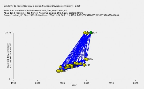
   There are two clusters of similarity. One cluster of size 20 spans from about year 2004 to 2010 with a similarity measure that increases in time from about five to ten. The other cluster of size three is dated near 2010 and has a similarity measure to the selected file of about 25.

   Files Program Files/Norton AntiVirus Engine 17.0.136 ccAlert.dll on drive

   AE10-1160 and Program Files/Norton AntiVirus Engine 17.8.0.5 on drive AE10

   -1147, which are the two yellow dots at the top of the figure, have significantly greater similarity of 25 than the other nodes that meet the similarity threshold. Two most recent

   
   

   of the less similar nodes, nodes 310 and 309, indicate AntiVirus Engine 16.8.0.41 and 16.0.0.125, so apparently version 16 was quite a bit different from version 17. The older files in this family are less similar and indicate a different versioning scheme or do not indicate a version number.

   Figure 5.7 shows the analysis of the edge that connects nodes 326 and 312, corresponding to Program Files/Norton AntiVirus Engine 18.5.0.125_ccalert.dll on drive AE10-1158 and Program Files Norton AntiVirus Engine 17.0.136_ccAlert.dll on drive AE10-1160. This display was obtained using the GUI by clicking on the edge shown in Figure 5.6 that connects these two files. The texture vector patterns appear very similar and the similarity histogram spikes with a similarity count of nearly 370 near file offset 0, a large number, indicating that these two files are similar. We can click on any of the yellow dots in the GUI to select the file corresponding to it to compare other files against it.

   
   

   

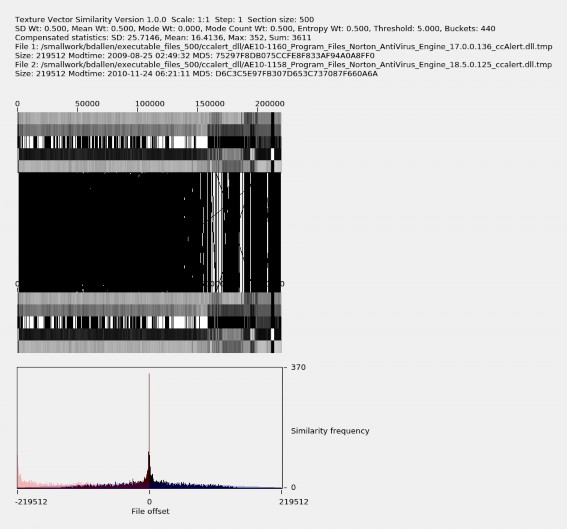
   Figure 5.7. A detailed comparison of files 312 and 326 showing a high degree of similarity.

   
   

   Figure 5.8 shows similarity of files within the powerpnt_exe file family to the Powerpoint file with the most recent timestamp in the dataset, file (node) 295. Not all files in this file family have version numbers in their names. By hovering the cursor over yellow dots representing files similar to node 295, we see files with a similarity measure of over 100 after year 2005 correspond to Microsoft Office 12, while less similar file (node) 303 has a similarity measure of about one near year 2003, and is labeled Microsoft Office 10.

   
   

   

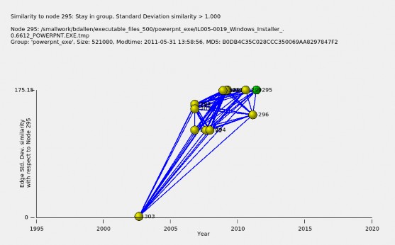
   Figure 5.8. Files similar to the latest Microsoft Office file in file family

   powerpnt_exe.

   
   

   Comparing nodes 326 and 310 for versions, which correspond correspond to Norton An- tiVirus Engine 18.5.0.125 and 16.8.0.41, we get the texture-vector graph shown in Figure 5.9. Here, there is more variance in the file offset, but the similarity frequency spikes to about 72, indicating that there is significant similarity. We also see more variation in the texture vector pattern and that the newer version is slightly larger in size, about 220 KB instead of 210 KB. By inspecting general changes in the five texture patterns, it appears that the additional 10 KB is inserted within the first 150 KB of the file.

   
   

   

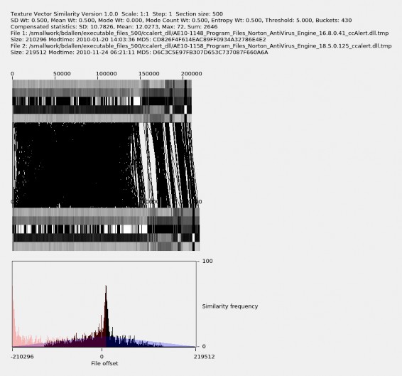
   Figure 5.9. Comparison of files 326 and 310.

   
   

   1. Composition Analysis

      By looking at the five bands in the texture-vector diagram, we can make inferences about the regions of executable code files being compared, in particular the locations of header, code, and data sections. For Figure 5.7, for the first two textures, covering the first 1,000 bytes, the standard deviation, mean, mode, and entropy values are lower than the values in other regions, while the mode count is higher. We infer that this represents a header, and the transition in the texture represents a transition to another type of content. The region

      
      

      from approximately byte 1,000 to byte 160,000, contains relatively medium values of the standard deviation, mean, and entropy, mode values that are either very high or very low, and consistently low mode counts. We infer that this is the code section. The third region, from approximately byte 160,000 through to the end at byte 219,512, usually has a low mode value while values in the other four statistics vary but consistently witht the two files. We infer that this is a region of data mostly unchanged between version. We also infer that the additional 10 KB added in the newer version was new code.

      
      

   2. Progressive Time Similarity

      Software files tend to be most similar to the previous version. Figure 5.10 shows an example for the nvrshu_dlll file family. Here, the file with the latest timestamp, WINDOWS system32 nvrshu.dll from the MY01-023 drive from Malaysia, is selected. We see sporatic measures of similarity between 10 and 30 for files before year 2005, but for files after 2005, we see a gradual increase in similarity over time from about 40 to 61.

      
      

      

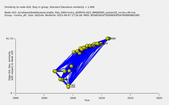
      Figure 5.10. Similarity increases as versions approach the latest version.

      
      

   3. Version Analysis

      With these diagrams, we can study on the origin and evolution of versions of files. Although an original file should have the earliest file creation time, file cre- ation times can be modified inadvertently or maliciously. Another clue is that the original file often has the least amount of code. Node 326 in Figure 5.6, file Program Files/Common Files/Symantex/Shared ccAlert.dll.tmpfrom drive PA002- 049 from Panama is likely the original file in its group because its file modification time is earliest and its similarity to latest files decreases over time.

      A newer version of code that introduces new features is likely to contain more code than the version before it as in Figure 5.9. A newer version that is only a bug fix will be similar in size to the version before it and will have similar texture-vector patterns as in Figure 5.7.

      Files released at approximately the same time may be targeted for different operating system platforms or different feature sets. For example 13 files in the webclnt_dll file family were released over two days, 2006-01-03 and 2006-01-04. This is too clustered to be in response to new functionality or bug fixes. These files could be a response to a virus because some of their file sizes are the same and their texture-vector patterns appear identical. However, bear in mind our sample is incomplete and important versions of software may be missing.‌

      
      

4. Examining Similarity using Gephi

Although the Texture-Vector Browser GUI tool was specifically designed for examining network graphs created from the dataset of similarity-graph files, graph analytics can also be done with popular open-source tools such as the Gephi graph-visualization tool. Steps for working with similarity-graph data using Gephi are presented in Appendix D.

CHAPTER 6:‌

Conclusions and Future Work

1. Conclusions‌

   This thesis proposed applying a vector of transforms to executable code to create texture- vector data, and then using analytics to identify similarities between executable files. We tested a sample of executable code files with our methods. Our experiments showed files within file families had greater average similarity than files across file families. We found that the visual patterns in the texture vectors were effective in identifying similar regions in two files as well as sections that may be compressed.‌

   
   

2. Future Work

   This work used texture vectors calculated from a section size of 500 bytes. A large section size might reveal similarity across a larger section of data, equivalent to applying a low-pass filter to texture-vector values. A section size that is a power of two or is aligned to the size of fixed-size data might naturally align better with the section boundaries from which texture-vectors are calculated.

   Texture vectors may be useful for classifying file types or detecting types of data embedded within a file. Further work in this direction might consist of defining data patterns that map to particular data types.

   The open-source tool Gephi offers many capabilities such as filtering and neighbor analytics that can be used to augment the similarity analytics provided by our tool. Future work might use it to obtain additional insight about file similarity.

   
   

   THIS PAGE INTENTIONALLY LEFT BLANK

   
   

   

   
   

   APPENDIX A:‌

   The Texture-Vector Similarity Toolset

   
   

   The Texture-Vector Similarity toolset bundles the previously mentioned features to provide a texture-vector approach for identifying similarities between files. While created for analyzing similarity between executable files, it can identify similarities in other file types. The Texture-Vector Similarity distribution, which bundles the toolset with sample data and other analytics tools, provides the following:

   • The calc_tv.py tool for calculating texture-vector files

   • The tv.py tool for calculating similarity metrics between two texture-vector files

   • The tv_browser.py tool for examining the similarity-graph dataset

   • Miscellaneous programs for organizing the dataset and calculating statistics from it

   • The texture-vector and similarity-graph dataset

The distribution has of approximately 3,300 lines of code in 65 files. It is primarily written in Python and uses the Qt 5 GUI widget toolkit for its graphical interface. Usage for these tools is presented in Appendix A.2 and source code for these tools is presented in Appendix E. Texture-vector files are described in Appendix C, and similarity-graph files are described in Appendix D.

Users interested in examining similarity between files that are not included in our dataset are encouraged to do so by running the calc_tv.py and tv.py tools directly.

Users who wish to analyze texture-vector files with their own tools can use the Texture- Vector Generator tool to create files in JSON format describing the file metadata, the section size used, the texture-vector labels, and the texture vectors as described in Appendix C.‌

1. Download

   The Texture-Vector Similarity toolset and requisite texture-vector datasets are publicly avail- able on the GitHub repository at https:// github.com/ NPS-DEEP/ tv_sim. Clone or download the Texture-Vector Similarity toolset from this site. For license information, please see the COPYING file in this repository or refer to Appendix E.4.

   
   

   The repository includes the following:

   • The Texture-Vector Similarity toolset.

   • .tv Texture Vector files calculated from Windows .exe and .dll executable code using default settings.

   • Node and Edge graph data.

   • Miscellaneous Python code used for generating .tv and graph data.

     The repository does not include any Windows .exe and .dll executable code from which the .tv files were generated.

     The following Linux example clones the Texture-Vector Similarity toolset into the gits/

     subdirectory under your home path:

     • mkdir ~/gits

     • cd ~/gits

     • git clone https://github.com/NPS-DEEP/tv_sim

       If you are a Windows user, you may prefer to download the ZIP file from https:// github. com/ NPS-DEEP/ tv_sim and extract it into a directory of your choosing.

       These tools require Python3, numpy, scipy, and PyQt5.

       • Windows users: To see if Python3 is present, open a command window and type python and look for Python3 in the response. Once Python is installed, open a command window and type:

         • python -m pip install PyQt5 numpy scipy

       • Mac/Linux users: To see if Python3 is present, open a command window and type python3 and look for Python3 in the response. Once Python is installed, open a command window and type:

         • python3 -m pip install PyQt5 numpy scipy‌

           
           

2. Usage

All tools in the Texture-Vector Similarity toolset are in the python subdirectory. For example if you installed the toolset under ~/gits, the tools will be at ~/gits/tv_sim/python.

You select the python subdirectory so that the tools may be run directly:

• cd ~/gits/tv_sim/python

  
  

  1. Texture-Vector Generator

     The Texture-Vector Generator tool calculates texture vectors as described in Chapter 3.1. Parameters are:

     • The input filename.

     • The output filename, which defaults to the input filename plus extension .tv.

     • The section size, which defaults to 500.

       Here is the usage for this tool:

       
       

       usage: calc_tv.py [-h] [-o OUTPUT_FILENAME] [-s SECTION_SIZE] filename Calculate texture vectors for a file.

       positional arguments:

       filename The input file.

       
       

       optional arguments:

       -h, --help show this help message and exit

       -o OUTPUT_FILENAME, --output_filename OUTPUT_FILENAME

       An alternate output filename, default is

       <filename>.tv.

       -s SECTION_SIZE, --section_size SECTION_SIZE

       The section size of the texture sample, default 500.

       
       

       Run the Texture-Vector Generator by typing the following:

• ./calc_tv your_filename

  where your_filename is the name of the file you would like to calculate texture vectors for.

  
  

  1. Texture-Vector Similarity GUI

     The Texture-Vector Similarity GUI tool provides a GUI for examining similarity between two texture vector files calculated via the Texture-Vector Generator tool as described in Chapter 3.4. Optional parameters are:

     • An alternate texture-vector threshold-settings file.

     • Sketch-step granularity to enable faster performance by skipping datapoints.

     • A flag to output to a default .jpg file instead of starting the GUI.

     • A flag to output to a named .jpg file instead of starting the GUI.

       Here is the usage for this tool:

       
       

       usage: tv.py [-h] [-s TV_THRESHOLD_SETTINGS_FILE] [-g] [-z ZOOM_COUNT] [-o | -n NAMED_OUTPUT | -m]

       [file1] [file2]

       GUI for graphing Texture Vector similarity. positional arguments:

       file1 The first .tv file to compare with.

       file2 The second .tv file to compare with.

       
       

       optional arguments:

       -h, --help show this help message and exit

       -s TV_THRESHOLD_SETTINGS_FILE, --tv_threshold_settings_file TV_THRESHOLD_SETTINGS_FILE A texture vector threshold settings file to use.

       -g, --sketch_granularity

       Use faster sketch step granularity.

       -z ZOOM_COUNT, --zoom_count ZOOM_COUNT

       Number of times to zoom in.

       -o, --output Output graph to default filename instead of showing a GUI.

       -n NAMED_OUTPUT, --named_output NAMED_OUTPUT

       Output graph to named file instead of showing a GUI.

       -m, --sd_metric Print the standard deviation metric instead of showing a GUI.

       
       

       Start the GUI by typing:

       
       

• ./tv.py

  The available toolbar actions are:

  • Open1 selects .tv file 1.

  • Open2 selects .tv file 2.

  • Settings opens a settings dialog box as shown in Figure A.1.

    
    

    

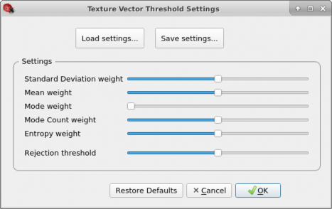
    Figure A.1. Example Texture-Vector Similarity GUI settings dialog.

    
    

    Adjusting texture-vector threshold sensitivity settings affects the view in real time. Settings may be loaded or saved using settings files. Settings selections persist between sessions in the user’s home directory in file ~/.tv_threshold_settings. The settings selection will be unselected when you close the settings dialog window unless you click OK.

  • Sketch selects sketch mode, which improves rendering performance for large files at the cost of detail and accuracy. We recommend using sketch mode for files larger than 10MB in size. Sketch mode improves performance by using a step rate of 50 so that only 1 in 50 texture vectors of each file are compared, resulting in a 50 ∗ 50 = 2, 500X speedup, providing a quick but less accurate representation of similarity.

    • + zooms the texture-vector plot in.

  • - zooms the texture-vector plot out.

    
    

  • 1 restores the texture-vector plot to its original scale of 1:1, meaning one pixel of space is used horizontally for every one texture vector calculated.

  • Export Graph exports the texture-vector graphics view as a .jpg image file.

    An example comparison of two versions of mobsync.exe is shown in Figure A.2.

    
    

    

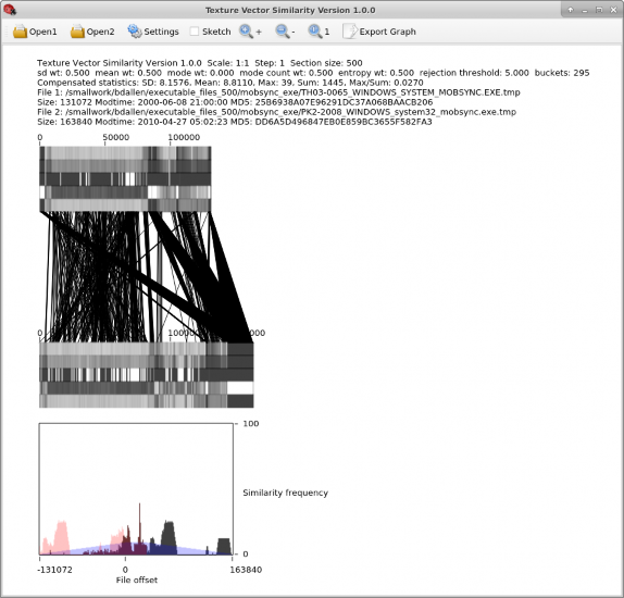
    Figure A.2. The Texture-Vector Similarity GUI showing similarity between two similar files.

    
    

    The top of the window shows information about the two files being compared:

    
    

  • The scale of the texture plot, in this case 1:1,

  • The step rate across the texture vectors, in this case 1.

  • The section size used for calculating the texture vectors, in this case the default size of 500 bytes.

  • The similarity weights used for determining texture similarity. Here, default weights presented in Chapter 4.3 are used.

  • The similarity statistics calculated from the compensated histogram described in Chapter3.3. These statistics include the histogram’s standard deviation, mean, maxi- mum value, and sum.

  • Information about the two files being compared including their filename, size, file modification time, and MD5 cryptographic hash.

    The middle of the figure graphs the texture vectors of the two files, along with similarity lines indicating locations of similarity between the two files.

    The bottom section graphs the similarity offset histograms. All three histograms described in Chapter3.3 are shown because each one provides useful information about similarity.

    
    

    1. Usage Example

       Here is an example of comparing two large (approximately 20MB each) files named

       Adobe_Reader_9.0.dll and Adobe_Reader_10.0.dll.

       1. Open a command window and change to the python directory. For example if you installed the Texture-Vector Similarity toolset at ~/gits then type:

          • cd /gits/tv_sim/python

       2. Run calc_tv.py to generate the texture-vector files Adobe_Reader_9.0.dll.tv and Adobe_Reader_10.0.dll.tv from Adobe_Reader_9.0.dll and Adobe_Reader_10.0.dll:

          • ./calc_tv.py Adobe_Reader_9.0.dll

          • ./calc_tv.py Adobe_Reader_10.0.dll

       3. Start the Texture-Vector Similarity GUI:

          • ./tv.py

       4. Because these files are larger than 10MB, press the Sketch button now to improve rendering performance in the next step when the files are opened, as recommended

          
          

          in Appendix A.2.2.

       5. Using the Open1 and Open2 buttons, load the two .tv texture-vector files generated above.

       6. Use the Settings button to tune similarity sensitivities if your existing settings are not suitable.

       
       

    2. Texture-Vector Browser GUI

       The Texture-Vector Browser GUI tool starts from the command line. Its optional parameter is the index of the file to start out as the selected file node.

       Here is the usage for this tool:

       
       

       usage: tv_browser.py [-h] [-i INDEX] TV file similarity browser.

       optional arguments:

       -h, --help show this help message and exit

       -i INDEX, --index INDEX

       The index of the first file to compare with.

       
       

       Run it by typing:

• ./tv_browser.py

  The available toolbar actions are:

  • Node opens a table of metadata about each of the files in the dataset. Each column in the table describes an item of metadata about a file. Each column may be sorted. Click on a row to select its file for browser analysis. Here are the columns of this table:

    • index: The graph node index assigned to this file.

    • filename: The name of the file associated with this node.

    • file_group: The similarity-based file group of the file associated with this node.

    • file_size: The size, in bytes, of the file associated with this node.

      
      

    • modtime: The modification time of the file associated with this node.

    • file_md5: The MD5 cryptographic hash of the file associated with this node.

    The node table is shown in Figure A.3.

    
    

    

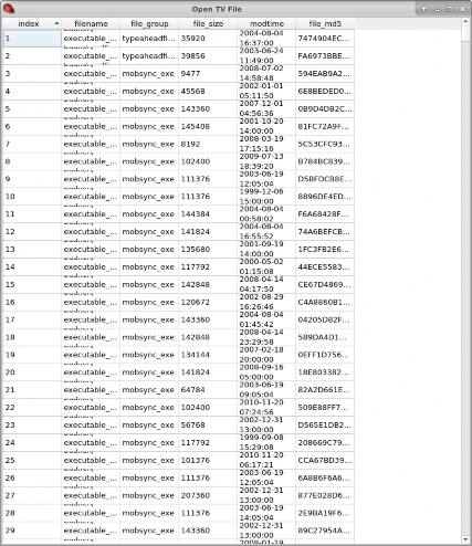
    Figure A.3. The TV file selection table.

    
    

  • Edge opens a table of metadata about similarity edges. The set of edges depends on the selected file node, whether the node neighbors are only in the selected file group, and the level of similarity required in order to show similarity edges between similar nodes. Each column in the table describes an item of metadata about an edge. Each column may be sorted. Click on a row to select the edge’s two files for further similarity analysis. Here are the columns of this table:

    • index1: The graph node index 1 associated with the edge. This index will be

      
      

      smaller than index 2

    • index2: The graph node index 2 associated with the edge.

    • sd: The standard deviation of the compensated histogram.

    • mean: The mean of the compensated histogram.

    • max: The maximum histogram bar value in the compensated histogram.

    • sum: The sum of the histogram bar values in the compensated histogram.

    For a description of the columns describing statistical properties please see Chap- ter 3.4.

    An example edge table for file node 10 is shown in Figure A.4.

    
    

    

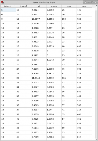
    Figure A.4. The similarity edge selection table for file node 10.

    
    

  • The Stay-in-group checkbox says whether to show only node neighbors in the selected

    
    

    file group.

  • The SD slider controls the level of similarity in standard deviation of the compensated histogram required in order to show similarity edges between similar nodes. Edges below this threshold will not be shown.

    • + zooms the similarity graph in.

  • - zooms the similarity graph out.

  • 1 restores the similarity graph to its original scale.

  • Export Graph exports the browser graph as a .jpg image file.

    An example view of the Texture-Vector Browser GUI with file node 79 selected is shown in Figure A.5. Not all nodes and edges associated with node 79 and its neighbors are shown. In this example, associated nodes and edges are restricted by the following constraints:

  • Only file nodes in file node 79’s file group are shown because the Stay in group

    checkbox is selected.

  • Only nodes with a similarity standard deviation of at least 1.000 and only edges with a similarity standard deviation of at least 1.000 are shown because the similarity SD threshold slider is set to select a minimum similarity standard deviation of 1.000.

    
    

    

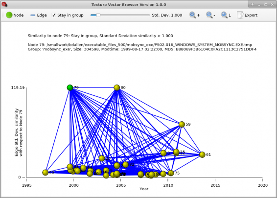
    Figure A.5. The Texture-Vector Browser GUI showing file node 79 selected.

    
    

    The upper part of the window shows file information about selected file node 79.

    The lower part of the window shows the graph of node 79 and all its neighbor nodes that are within its file group, with a standard deviation similarity measure of at least 1 standard deviation:

  • The selected node file is green.

  • All neighbor node files are yellow.

  • All edges that match with a similarity of at least 1 standard deviation are shown and are blue.

  • The horizontal axis identifies the modification time of the file associated with that node.

  • The vertical axis identifies the standard deviation similarity between a given node and the selected node.

    
    

    You may manipulate this graph and examine similarity between files:

  • Hover over a node to observe its associated file properties.

  • Click on a node to select it as the primary node.

  • Click on the primary node to view it in Texture-Vector Similarity GUI window.

  • Hover over an edge to observe the similarity information and file properties of the two files that the edge connects.

  • Click on an edge to view its texture-vector graph in a Texture-Vector Similarity GUI

    window.‌

    
    

    1. Texture-Vector Similarity Toolset Data

    Data in the Texture-Vector Similarity toolset consists of:

    • The set of 1,134 texture-vector files (.tv files) in directory tv_sim/python/sbatch_tv_t500. These files contain texture vectors calculated along 500 byte intervals and are named according to the MD5 cryptographic hash of the executable files they were obtained

      from. See Appendix C for the syntax of these files.

    • The node and edge files that comprise the similarity-graph of the dataset. These files

      are named nodes.csv and edges.csv and are in directory tv_sim/python/sbatch_graph_500. They correspond to the texture-vector files in directory tv_sim/python/sbatch_tv_t500.

      See Appendix D for the syntax of these files.

      
      

      THIS PAGE INTENTIONALLY LEFT BLANK

      
      

      

      
      

      APPENDIX B:‌

      Texture-Vector Threshold Settings

      
      

      Texture vector threshold settings set the acceptance thresholds for establishing texture vector similarity.

      The texture vector threshold settings file is in JSON format and defines the names of the texture vector algorithms, which of them are used, and their acceptance threshold values of each.

      Here is the texture vector threshold settings file showing default settings:

      
      

      {

      "sd_weight": 0.5,

      "mean_weight": 0.5,

      "mode_weight": 0.0,

      "mode_count_weight": 0.5,

      "entropy_weight": 0.5,

      "rejection_threshold": 50

      }

      
      

      THIS PAGE INTENTIONALLY LEFT BLANK

      
      

      

      
      

      APPENDIX C:‌

      Texture Vector Data Syntax

      
      

      The Texture-Vector Generator tool creates texture vector output in JSON format. This output consists of file metadata, the section size used, the texture vector labels, and the list of texture vectors. You may perform your own post-processing of texture vector files by reading and processing this data.

      Here is a description of the fields in the texture vector data:

    • version The version of the Texture-Vector Similarity toolset used to create the texture vector data.

    • filename The name of the file the texture vector data was created from.

    • file_size The size of the file the texture vector data was created from.

    • file_modtime The file modification timestamp of the file the texture vector data was created from.

    • md5 The MD5 hashcode of the file the texture vector data was created from.

    • section_size The size of the sections used by the transforms when calculating texture vector values.

    • texture_names The names of the texture vector transforms, in order.

    • texture_vectors The list of texture vectors, in order, where each texture vector is a list, in order, of texture vector element values.

    Here is an example fragment of a texture vector file named sort:

    
    

    {

    "version": "0.0.13",

    "filename": "sort", "file_size": 113120,

    "file_modtime": 1552008687.5194707,

    "md5": "33D8447AD6ED6C088B46C7A481F961F1",

    "section_size": 500, "texture_names": [

    "sd",

    "mean",

    
    

    "mode", "mode_count", "entropy"

    ],

    "texture_vectors": [ [

    84.45348172810876,

    14.066,

    0,

    196.608,

    56.0

    ], [

    135.22527598049115,

    45.428,

    0,

    136.704,

    125.0

    ],

    ]

    }

    
    

    
    

    

    
    

    APPENDIX D:‌

    Similarity-Graph Data Syntax

    
    

    The similarity graph is contained in a nodes file and an edges file, both in comma separated values (CSV). Here are the first few lines of the nodes file:

    
    

    Id,Name,Group,Size,Modtime,MD5,SectionSize

    ,,,,,,,Combinations from /smallwork/bdallen/tv_files/*.tv

    ,,,,,,,1294 files, 836571 combinations 1,/smallwork/bdallen/executable_files/typeaheadfind_dll/PS01-067_Program_Files_N etscape_Netscape_components_typeaheadfind.dll.tmp,typeaheadfind_dll,39856,105648 0540,FA6973BBE89049A6D1D3509F95ED9CF5,500

    2,/smallwork/bdallen/executable_files/typeaheadfind_dll/IL3-0205_Program_Files_N etscape_Netscape_components_typeaheadfind.dll.tmp,typeaheadfind_dll,35920,109166 2620,7474904ECFD547B29CB9F3D8B2CF0C40,500

    3,/smallwork/bdallen/executable_files/mobsync_exe/DE001-0003_WINDOWS_system32_dl lcache_mobsync.exe.tmp,mobsync_exe,8192,1205972116,5C53CFC93F332B109B2497ED38B51 F25,500

    
    

    Here are the first few lines of the edges file:

    
    

    Source,Target,SD,Mean,Max,Sum

    ,,,,,,Combinations from /smallwork/bdallen/tv_files/*.tv

    ,,,,,,1294 files, 836571 combinations

    1,2,2.4603,2.6500,12,212

    1,4,0.1118,0.0125,1,1

    5,1,0.6550,0.4615,2,42

    1,7,0.3651,0.1171,2,24

    8,1,0.4356,0.1480,2,33

    1,9,0.4136,0.1415,2,29

    10,1,0.4698,0.1737,3,41

    
    

    Similarity-graph node and edge files are compatible for direct input to the Texture-Vector Browser GUI tool and to graph tools such as the Gephi graph-visualization tool. Gephi graph visualization can be applied as follows:

    
    

    1. Open Gephi.

    2. Open the nodes file, for example open python/sbatch_graph_500/nodes.csv from the Texture-Vector Similarity toolset. This loads the graph node data. Gephi will correctly identify the column names and column types. Records 1 and 2 will be flagged as severe issues. They are not; they are just comment lines.

    3. Now open the edges file, for example open python/sbatch_graph_500/edges.csv from the Texture-Vector Similarity toolset. Select Append to existing workspace rather than the default New workspace to connect these edges with the nodes opened in the previous step. Gephi will correctly identify the column names and column types. Records 1 and 2 will be flagged as severe issues. They are not; they are just comment lines.

    4. Manipulate the graph view by selecting filters, weights, thresholds, etc., as desired.

    
    

    

    
    

    APPENDIX E:‌

    Source Code

    
    

    All source code is available online from GitHub at https:// github.com/ NPS-DEEP/ tv_sim. This chapter describes key components of this source code.‌

    
    

    1. Texture-Vector Similarity Source Code

       Several components of the Texture-Vector Similarity source code are shared between its tools. Here is a brief overview of these components:

       • Filenames starting with tv_ specifically support the Texture-Vector Similarity GUI.

       • Filenames starting with browser_ specifically support the Texture-Vector Browser GUI.

       • Filenames with _main_window are main windows.

       • Filenames with _widget are GUI widgets.

       • Filenames with _g_ are QGraphicsItem components.

       • Filenames with export_ export graphs to .jpg files.

       • The data_manager.py file reads and parses .tv files into data structures.

       • Filenames with settings_ relate to similarity settings.

       • File settngs_dialog.ui defines the settings window and is built using QT Designer 5.

       • Use file Makefile to build file settngs_dialog.py which is auto-generated and to update the version.

       • File version_file.py contains the version of the Texture-Vector Similarity toolset. It is auto-generated by the Makefile. Update the version in the Makefile and run make to update the version of the Texture-Vector Similarity toolset.

    Of special interest is the function for calculating texture vectors and the function for calcu- lating texture vector similarity. These functions are presented here.

    
    

    1. Calculating Texture Vectors

       The math behind calculating texture vectors is managed in function calc_tv in file

       calc_tv.py. This function takes the following parameters:

       • The input filename of the file to calculate texture vectors for.

       • The output filename of the file to write the calculated JSON TV data to.

       • The section size to use for calculating the texture vectors.

         The data structure generated and written in JSON format is described in Appendix C. Here is the source code listing for file calc_tv.py:

         # ! / usr / b i n / env python 3

         # r e q u i r e s numpy : " sudo p i p 3 i n s t a l l numpy "

         
         

         import sys , os , h a s h l i b

         from a r g p a r s e import Argument Parser

         import numpy as np

         import j s o n

         from math import e , lo g

         from v e r s i o n _ f i l e import VERSION

         t e x t u r e _ n a m e s =( " sd " , " mean " , " mode " , " mode_ count " , " e n t r o p y " )

         
         

         # use _ entropy 2 i n s t e a d

         def _ s h a n n o n 2 _ e n t r o p y ( b ) :

         # h t t p s : / / s t a c k o v e r f l o w . com / q u e s t i o n s / 42683287 / python −numpy−shannon − # entropy − array ? rq=1

         b_sum = b . sum ( ) i f b_sum == 0 : return 0

         p=b / b . sum ( )

         p r i n t ( np . lo g 2 ( p ) )

         shannon 2 =−np . sum ( p∗np . lo g 2 ( p ) )

         return shannon 2 . i t em ( )

         
         

         # from h t t p s : / / s t a c k o v e r f l o w . com / q u e s t i o n s / 15450192 / f a s t e s t −way− to −compu # t e − entropy − in − python approach 2

         def _ e n t r o p y 2 ( l a b e l s , b as e =None ) :

         " " " Computes en t r opy o f l a b e l d i s t r i b u t i o n . " " "

         
         

         n _ l a b e l s = l e n ( l a b e l s )

         i f n _ l a b e l s <= 1 :

         return 0

         
         

         value , c o u n t s = np . u n iq u e ( l a b e l s , r e t u r n _ c o u n t s = True ) p r o b s = c o u n t s / n _ l a b e l s

         n _ c l a s s e s = np . c o u n t _ n o n z e r o ( p r o b s )

         i f n _ c l a s s e s <= 1 :

         return 0

         e n t = 0 .

         
         

         # Compute en t r opy

         b as e = e i f b as e i s None e l s e b as e

         f o r i in p r o b s :

         e n t −= i ∗ lo g ( i , b as e )

         # quick o b s e r v a t i o n shows e n t between 0 . 0 and 4 . 0 .

         return e n t

         def _ t e x t u r e _ v e c t o r ( b , s e c t i o n _ s i z e ) :

         # t r y t o normalize f o r 0 t o 255 v a l u e s

         sd = np . s t d ( b ) . i t em ( ) ∗ 2 # s t andard d e v i a t i o n

         mean = np . mean ( b ) . i t em ( ) # mean

         # h t t p s : / / s t a c k o v e r f l o w . com / q u e s t i o n s / 6252280 / f i nd − the −most − f r e q u e n t #−number − in −a−numpy− v e c t o r

         mode = np . argmax ( np . b i n c o u n t ( b ) ) . i t em ( ) # mode

         mode_ count = l i s t ( b ) . c o u n t ( mode ) ∗ ( 2 5 6 . 0 / s e c t i o n _ s i z e ) # mode_ count

         # en t r opy = _ shannon 2 _ entropy ( b ) # en t r opy

         e n t r o p y = round ( _ e n t r o p y 2 ( b ) ∗ 43 ) # en t r opy

         return ( sd , mean , mode , mode_ count , e n t r o p y )

         def c a l c _ t v ( i n f i l e , o u t f i l e , s e c t i o n _ s i z e ) :

         # p r i n t ( " Preparing ’% s ’ from ’% s ’"%( o u t f i l e , i n f i l e ) )

         
         

         # t e x t u r e v e c t o r s

         
         

         t e x t u r e _ v e c t o r s = l i s t ( )

         
         

         # c a l c u l a t e s e c t i o n s

         o f f s e t =0

         f i l e _ s i z e = os . s t a t ( i n f i l e ) . s t _ s i z e

         f i l e _ m o d t im e = i n t ( os . p a t h . getmtime ( i n f i l e ) )

         md5 = h a s h l i b . md5 ( open ( i n f i l e , " rb " ) . r e a d ( ) ) . h e x d i g e s t ( ) . upper ( ) mod_ s ize = s e c t i o n _ s i z e ∗ 1000

         with open ( i n f i l e , mode= ’ rb ’ ) as f :

         while True :

         i f o f f s e t % mod_ s ize == 0 :

         p r i n t ( " P r o c e s s i n g u%du of u%d . . . "%( o f f s e t , f i l e _ s i z e ) ) b= f . r e a d ( s e c t i o n _ s i z e )

         i f not b :

         break

         d=np . f r o m b u f f e r ( b , d t y p e = ’ u i n t 8 ’ ) # b i nary array t o numpy data

         t e x t u r e _ v e c t o r s . append ( _ t e x t u r e _ v e c t o r ( d , s e c t i o n _ s i z e ) ) o f f s e t += l e n ( b )

         
         

         # save t e x t u r e v e c t o r f i l e

         j s o n _ t v = d i c t ( )

         j s o n _ t v [ " v e r s i o n " ]=VERSION j s o n _ t v [ " f i l e n a m e " ]= i n f i l e

         j s o n _ t v [ " f i l e _ g r o u p " ]= os . p a t h . basename ( os . p a t h . dirname ( i n f i l e ) ) j s o n _ t v [ " f i l e _ s i z e " ]= f i l e _ s i z e

         j s o n _ t v [ " f i l e _ m o d t im e " ]= f i l e _ m o d t im e j s o n _ t v [ " md5 " ]= md5

         j s o n _ t v [ " s e c t i o n _ s i z e " ]= s e c t i o n _ s i z e

         j s o n _ t v [ " t e x t u r e _ n a m e s " ] = t e x t u r e _ n a m e s

         j s o n _ t v [ " t e x t u r e _ v e c t o r s " ] = t e x t u r e _ v e c t o r s with open ( o u t f i l e , "w" ) as f :

         j s o n . dump ( j s o n _ t v , f , i n d e n t = 4 )

         
         

         i f __name__==" __ main__ " :

         p a r s e r = Argument Parser ( prog = ’ c a l c _ t v . py ’ ,

         d e s c r i p t i o n =" C a l c u l a t e u t e x t u r e u v e c t o r s u f o r u a u f i l e . " )

         p a r s e r . add_ argument ( " f i l e n a m e " , type = s t r , help =" Theu i n p u t u f i l e . " ) p a r s e r . add_ argument ( "−o " , "−− o u t p u t _ f i l e n a m e " , type = s t r ,

         
         

         help ="Anu a l t e r n a t e u o u t p u t u f i le n a m e , u d e f a u l t u i s u

         < f i le n a m e > . t v . " )

         p a r s e r . add_ argument ( "−s " , "−− s e c t i o n _ s i z e " , type = i n t , d e f a u l t = 500 ,

         help =" Theu s e c t i o n u s i z e u of u t h e u t e x t u r e u sample , u d e f a u l t u 5 0 0 . " )

         a r g s = p a r s e r . p a r s e _ a r g s ( )

         s e c t i o n _ s i z e = a r g s . s e c t i o n _ s i z e

         i f s e c t i o n _ s i z e < 1 :

         p r i n t ( " I n v a l i d u s e c t i o n u s i z e u%s "%s e c t i o n _ s i z e ) s y s . e x i t ( 1 )

         i n f i l e = a r g s . f i l e n a m e

         i f not os . p a t h . i s f i l e ( i n f i l e ) :

         p r i n t ( " E r r o r : u In p u t u f i l e u’% s ’ u does u n o t u e x i s t . "% i n f i l e ) s y s . e x i t ( 1 )

         i f a r g s . o u t p u t _ f i l e n a m e :

         o u t f i l e = a r g s . o u t p u t _ f i l e n a m e

         e l s e :

         o u t f i l e = "%s . t v "% i n f i l e

         i f os . p a t h . e x i s t s ( o u t f i l e ) :

         p r i n t ( " E r r o r : u Output u f i l e u’% s ’ u a l r e a d y u e x i s t s . "%o u t f i l e ) s y s . e x i t ( 1 )

         
         

         p r i n t ( " P r e p a r i n g u’% s ’ u from u’% s ’ "%( o u t f i l e , i n f i l e ) ) c a l c _ t v ( i n f i l e , o u t f i l e , s e c t i o n _ s i z e )

         p r i n t ( " Done . " )

         
         

    2. Calculating Texture Similarity

       The math behind calculating texture vector similarity is managed in function generate_similarity_data in file similarity_math.py. This function takes the following parameters:

       • Texture Vector Dataset 1.

       • Texture Vector Dataset 2.

       • The step interval for large files, if optimization is required, or 1 for no optimization.

       • The similarity settings to use for defining similarity thresholds, see Chapter 4.3. and Appendix B.

       • Whether similarity lines need calculated (the function runs faster if similarity lines

         
         

         do not need to be calculated).

         The data structure returned includes the similarity histogram and statistics calculated from this histogram, all of which may be used as similarity metrics.

         Here is the source code listing for file similarity_math.py:

         from c o l l e c t i o n s import d e f a u l t d i c t

         from math import c e i l , f l o o r

         from s c i p y . s p a t i a l . d i s t a n c e import e u c l i d e a n

         import s t a t i s t i c s

         
         

         " " "

         C a l c u l a t e s s i m i l a r i t y l i n e s , h i s t ograms , and s t a t i s t i c s . " " "

         
         

         # Return compensated h i s t ogram where t h e r i g h t s l o p e p a r t i s f l i p p e d # and added t o t h e l e f t s l o p e p a r t .

         def _ c o m p e n s a t e d _ h i s t o g r a m ( s i z e 1 , s i z e 2 , h i s t o g r a m ) :

         i f s i z e 1 + s i z e 2 == 0 :

         return l i s t ( ) , l i s t ( )

         
         

         # ordered s i z e l a r g e = s i z e 1 s m a l l = s i z e 2

         i f s m a l l > l a r g e :

         l a r g e , s m a l l = small , l a r g e

         
         

         # number o f s l o p e b u c k e t s

         num_ buckets = l e n ( h i s t o g r a m )

         n u m _ l e f t _ s l o p e _ b u c k e t s = i n t ( num_ buckets ∗ s m a l l / ( l a r g e + s m a l l ) + 0 . 4 9 )

         
         

         # compensated h i s t ogram

         c o m p e n s a t e d _ h i s t o g r a m = h i s t o g r a m [: − n u m _ l e f t _ s l o p e _ b u c k e t s ] j = num_ buckets − n u m _ l e f t _ s l o p e _ b u c k e t s

         f o r i in range ( n u m _ l e f t _ s l o p e _ b u c k e t s ) :

         c o m p e n s a t e d _ h i s t o g r a m [ i ] += h i s t o g r a m [ j + i ]

         
         

         # mean power

         mean_power = s t a t i s t i c s . mean ( h i s t o g r a m ) max_mean_power = mean_power ∗ ( ( l a r g e + s m a l l ) / l a r g e ) mean_ power_ histogram = [ max_mean_power ] ∗ num_ buckets f o r i in range ( n u m _ l e f t _ s l o p e _ b u c k e t s ) :

         lo c a l_ m e a n = max_mean_power ∗ i / n u m _ l e f t _ s l o p e _ b u c k e t s mean_ power_ histogram [ i ] = lo c a l_ m e a n mean_ power_ histogram [ − i ] = lo c a l_ m e a n

         return c o m p e n s a t e d _ h i s t o g r a m , mean_ power_ histogram

         
         

         # g e t num_ buckets and s e c t i o n s _ p e r _ b u c k e t

         def _ b u c k e t _ i n fo ( s e c t i o n _ s i z e , s t e p , f i l e _ s i z e 1 , f i l e _ s i z e 2 ) :

         t o t a l _ s e c t i o n s = c e i l ( ( f i l e _ s i z e 1 + f i l e _ s i z e 2 ) / s e c t i o n _ s i z e ) s e c t i o n s _ p e r _ b u c k e t = c e i l ( t o t a l _ s e c t i o n s / s t e p / 500 ) ∗ s t e p num_ buckets = c e i l ( t o t a l _ s e c t i o n s / s e c t i o n s _ p e r _ b u c k e t )

         n u m _ f 1 _ s e c t io n s = f i l e _ s i z e 1 / s e c t i o n _ s i z e # f l o a t

         return num_ buckets , s e c t i o n s _ p e r _ b u c k e t , n u m _ f 1 _ s e c t io n s

         
         

         # f o r compensated h i s t ogram

         def _ h i s t o g r a m _ s t a t s ( h i s t o g r a m ) :

         # h i s t ogram mean and SD , SD r e q u i r e s a t l e a s t 2 data p o i n t s

         i f l e n ( h i s t o g r a m ) >= 2 :

         sd = s t a t i s t i c s . s t d e v ( h i s t o g r a m ) mean = s t a t i s t i c s . mean ( h i s t o g r a m ) maxv = max ( h i s t o g r a m )

         sumv = sum ( h i s t o g r a m )

         e l s e :

         sd = 0 . 0

         mean = 0 . 0

         maxv = 0

         sumv = 0

         return sd , mean , maxv , sumv

         
         

         def e m p t y _ s i m i l a r i t y _ d a t a ( ) : empty_ data = d i c t ( )

         empty_ data [ " s i m i l a r i t y _ l i n e s " ] = d i c t ( ) empty_ data [ " s i m i l a r i t y _ h i s t o g r a m " ] = l i s t ( ) empty_ data [ " c o m p e n s a t e d _ h i s t o g r a m " ] = l i s t ( ) empty_ data [ " mean_ power_ histogram " ] = l i s t ( )

         
         

         empty_ data [ " sd " ] = 0 . 0 empty_ data [ " mean " ] = 0 . 0 empty_ data [ " max" ] = 0 empty_ data [ " sum " ] = 0 return empty_ data

         
         

         # r e t u r n data s t r u c t u r e s g i v en i n p u t s

         def g e n e r a t e _ s i m i l a r i t y _ d a t a ( t v _ d a t a 1 , t v _ d a t a 2 , s t e p ,

         s e t t i n g s , u s e _ s i m i l a r i t y _ l i n e s ) :

         
         

         # v a l i d a t e i n p u t

         i f not t v _ d a t a 1 or not t v _ d a t a 2 :

         # no data

         return e m p t y _ s i m i l a r i t y _ d a t a ( )

         i f not t v _ d a t a 1 [ " s e c t i o n _ s i z e " ] == t v _ d a t a 2 [ " s e c t i o n _ s i z e " ] :

         r a i s e E x c e p t io n ( " In c o m p a t i b l e u t v u d a t a : u s e c t i o n u s i z e u mismatch . " )

         i f s t e p < 1 :

         r a i s e E x c e p t io n ( " Bad " )

         
         

         # c a l c u l a t e bucket numbers f o r even s e c t i o n d i s t r i b u t i o n

         num_ buckets , s e c t i o n s _ p e r _ b u c k e t , n u m _ f 1 _ s e c t io n s = _ b u c k e t _ i n fo (

         t v _ d a t a 1 [ " s e c t i o n _ s i z e " ] , s t e p , t v _ d a t a 1 [ " f i l e _ s i z e " ] ,

         t v _ d a t a 2 [ " f i l e _ s i z e " ] )

         
         

         # s i m i l a r i t y l i n e s and s i m i l a r i t y h i s t ogram

         s i m i l a r i t y _ l i n e s = d e f a u l t d i c t ( l i s t )

         s i m i l a r i t y _ h i s t o g r a m = [ 0 ] ∗ num_ buckets

         
         

         # o p t i m i z a t i o n

         r e j e c t i o n _ t h r e s h o l d = s e t t i n g s [ " r e j e c t i o n _ t h r e s h o l d " ] w0 = s e t t i n g s [ " s d _ w e ig h t " ]

         w1 = s e t t i n g s [ " mean_ weight " ] w2 = s e t t i n g s [ " mode_ weight " ]

         w3 = s e t t i n g s [ " mode_ count_ weight " ] w4 = s e t t i n g s [ " e n t r o p y _ w e ig h t " ] w=[w0 , w1 , w2 , w3 , w4 ]

         
         

         i f sum (w) == 0 . 0 :

         return e m p t y _ s i m i l a r i t y _ d a t a ( )

         
         

         d a t a 1 = t v _ d a t a 1 [ " t e x t u r e _ v e c t o r s " ] d a t a 2 = t v _ d a t a 2 [ " t e x t u r e _ v e c t o r s " ]

         
         

         # h i s t ogram numbers

         f i l e _ s i z e 1 = t v _ d a t a 1 [ " f i l e _ s i z e " ] f i l e _ s i z e 2 = t v _ d a t a 2 [ " f i l e _ s i z e " ]

         s e c t i o n _ s i z e = t v _ d a t a 1 [ " s e c t i o n _ s i z e " ]

         
         

         # f i n d s i m i l a r i t y l i n e s

         f o r i in range ( 0 , l e n ( d a t a 1 ) , s t e p ) : v1 = d a t a 1 [ i ]

         f o r j in range ( 0 , l e n ( d a t a 2 ) , s t e p ) : v2 = d a t a 2 [ j ]

         d= e u c l i d e a n ( v1 , v2 , w)

         i f d > r e j e c t i o n _ t h r e s h o l d :

         c o n t i n u e

         
         

         # maybe add p o i n t t o s i m i l a r i t y l i n e s

         i f u s e _ s i m i l a r i t y _ l i n e s :

         s i m i l a r i t y _ l i n e s [ i ] . append ( j )

         
         

         # add p o i n t t o s i m i l a r i t y h i s t ogram

         b u c k e t = i n t ( ( j − i + n u m _ f 1 _ s e c t io n s ) / s e c t i o n s _ p e r _ b u c k e t )

         s i m i l a r i t y _ h i s t o g r a m [ b u c k e t ] += 1

         
         

         # prepare compensated and mean power h i s t ograms

         c o m p e n s a t e d _ h i s t o g r a m , mean_ power_ histogram =

         _ c o m p e n s a t e d _ h i s t o g r a m (

         f i l e _ s i z e 1 , f i l e _ s i z e 2 , s i m i l a r i t y _ h i s t o g r a m )

         
         

         # prepare h i s t ogram s t a t i s t i c s

         sd , mean , maxv , sumv = _ h i s t o g r a m _ s t a t s ( c o m p e n s a t e d _ h i s t o g r a m )

         
         

         # b u i l d s i m i l a r i t y data s i m i l a r i t y _ d a t a = d i c t ( ) i f u s e _ s i m i l a r i t y _ l i n e s :

         s i m i l a r i t y _ d a t a [ " s i m i l a r i t y _ l i n e s " ] = s i m i l a r i t y _ l i n e s

         s i m i l a r i t y _ d a t a [ " s i m i l a r i t y _ h i s t o g r a m " ] = s i m i l a r i t y _ h i s t o g r a m

         
         

         s i m i l a r i t y _ d a t a [ " c o m p e n s a t e d _ h i s t o g r a m " ] = c o m p e n s a t e d _ h i s t o g r a m s i m i l a r i t y _ d a t a [ " mean_ power_ histogram " ] = mean_ power_ histogram

         s i m i l a r i t y _ d a t a [ " sd " ] = sd

         s i m i l a r i t y _ d a t a [ " mean " ] = mean s i m i l a r i t y _ d a t a [ " max" ] = maxv s i m i l a r i t y _ d a t a [ " sum " ] = sumv

         
         

         return s i m i l a r i t y _ d a t a

         
         

    1. Source Code for Batch Processing‌

       Due to the size of our data, we created batch processing tools to expedite calculating texture vector data and for calculating similarity data between files. These tools are presented here.

       
       

       1. Calculating Texture Vectors

          We calculate all texture vector files by running sbatch_calc_tv.bash as follows:

• sbatch sbatch_calc_tv.bash

  Program sbatch_calc_tv.bash is a program that runs on the Slurm workload manager and executes sbatch_calc_tv.py on multiple processors. Program sbatch_calc_tv.py calculates one texture vector file given an executable file to process. Program sbatch_calc_tv.py uses function calc_tv from file calc_tv.py to calculate the texture vector data for a given file.

  Output from the sbatch_calc_tv.py jobs consists of generated .tv files.

  
  

  1. Calculating Similarity Metrics

     We calculate similarity between all texture vector files by running sbatch_ddiff_tv.bash as follows:

• sbatch sbatch_ddiff_tv.bash

Program sbatch_ddiff_tv.bash is a program that runs on the Slurm workload manager and executes sbatch_ddiff_tv.py on multiple processors. Program sbatch_ddiff_tv.py calculates difference metrics for a given input file. Program sbatch_ddiff_tv.py uses

function similarity_math from file similarity_math.py to calculate difference met- rics between two files.

Output from each batch job is directed to a data file associated with that batch job. Each data file consists of similarity metric data formatted as CSV. Entries with zero similarity measure are skipped. The result of the run is one CSV file for nodes, and many CSV files for edges. When the run completes, we collate the edge files into one and make sure the edge titles are at the top of the file so that it is compatible for input to Gephi.

The syntax and composition of the node and edge CSV files are described in Appendix D.

1. Data Preparation

   Tools for preparing large sets of files and for assisting in validating correctness are in the

   sbatch_prep/ directory.‌

   
   

1. Source Code for Statistical Analysis

   Source code for various statistical analysis is available in the statistics/ directory.‌‌

   
   

2. Source Code License

All code is provided with the following notice:

The software provided here is released by the Naval Postgraduate School, an agency of the

U.S. Department of Navy. The software bears no warranty, either expressed or implied. NPS does not assume legal liability nor responsibility for a User’s use of the software or the results of such use.

Please note that within the United States, copyright protection, under Section 105 of the United States Code, Title 17, is not available for any work of the United States Government and/or for any works created by United States Government employees. User acknowledges that this software contains work which was created by NPS government employees and is therefore in the public domain and not subject to copyright.

THIS PAGE INTENTIONALLY LEFT BLANK

List of References

1. B. Kolosnjaji, A. Demontis, B. Biggio, D. Maiorca, G. Giacinto, C. Eckert, and

   F. Roli, “Adversarial malware binaries: Evading deep learning for malware detec- tion in executables,” in 26’th European Signal Processing Conference, Rome, Italy, December 2018, Proceedings.

2. S. Josse, E. Bachaalany, A. Gazet, and B. Dang, Practical Reverse Engineering: x86, x64, ARM, Windows Kernel, Reversing Tools, and Obfuscation, 1st ed. Indi- anapolis, IN: Wiley, 2014.

3. T. Arbuckle, “Visually summarising software change,” in 12th International Confer- ence Information Visualization, 2008.

4. E. Aghajani, A. Mocci, G. Bavota, and M. Lanza, “The code time machine,” in 2017 IEEE 25th International Conference on Program Comprehension (ICPC).

5. H. Koike and H.-C. Chu, “Vrcs: Integrating version control and module manage- ment using interactive three-dimensional graphics,” in Graduate School of Informa- tion Systems University of Elect ro-Communications Chofu, Tokyo 182, Japan, 1997.

6. L. Voinea, A. Telea, and J. J. van Wijk, “Cvsscan: Visualization of code evolution,” in SoftVis ’05 Proceedings of the 2005 ACM symposium on software visualization, 2005, pp. 47–56.

7. M. Burch, S. Diehl, and P. Weißgerber, “Visual data mining in software archives,” in SoftVis ’05 Proceedings of the 2005 ACM symposium on software visualization, 2005, pp. 37–46.

8. T. R. L. Bergroth, H. Hakonen, “A survey of longest common subsequence algo- rithms,” in Proc. Int’l Symp. String Processing Information Retrieval (SPIRE ’00), 2000, pp. 39–48.

9. Wikipedia. (Feb. 4, 2020). Knuth-Morris-Pratt algorithm. [Online]. Available: https:

   //en.wikipedia.org/wiki/Knuth-Morris-Pratt_algorithm. Accessed Feb. 11, 2020.

10. R. Cole, Tight Bounds on the Complexity of the Boyer-Moore Pattern Matching Al- gorithm, 1st ed. London: Forgotten Books, 2018.

11. W. Shotts, The Linux Command Line, 2nd ed. San Francisco, CA: No Starch Press, 2019.

    
    

12. D. Cabezas and B. Mooij, “Detecting source code re-use through a binary analy- sis hybrid approach,” accessed May 2, 2019. Available: https://www.forensicmag. com/article/2013/02/detecting-source-code-re-use-through-binary-analysis-hybrid- approach

13. J. Jang and D. Brumley, “Bitshred: Fast, scalable code reuse detection in binary code,” in CMU-CyLab-10-006, 2009.

14. N. C. Rowe, “Associating drives based on their artifact and metadata distributions,” in 10th International EAI Conference, ICDF2C 2018, New Orleans, LA, USA, September 10–12, 2018, Proceedings.

15. A. Hadmi, W. Puech, B. A. E. Said, and A. A. Ouahman, “Perceptual image hash- ing,” in University of Montpellier II, CNRS UMR 5506-LIRMM, France, 2012.

16. J. Seemann and J. W. von Gudenberg, “Visualization of differences between versions of object-oriented software,” in Proceedings of the Second Euromicro Conference on Software Maintenance and Reengineering, 11-11 March 1998, Florence, Italy, Italy.

17. J. Rho and C. Wu, “An efficient version model of software diagrams,” in Proceed- ings 1998 Asia Pacific Software Engineering Conference (Cat. No.98EX240), 2-4 Dec. 1988, Taipei, Taiwan, Taiwan.

18. W. Swierstra and A. Löh, “The semantics of version control,” in Proceedings of the 2014 ACM International Symposium on New Ideas, New Paradigms, and Reflections on Programming and Software (Onward! 2014), 43-54, New York, NY, USA.

19. A. Defant, Classical Summation in Commutative and Noncommutative Lp-Spaces, 1st ed. New York, NY: Springer, 2011.

20. S. Garfinkel, P. Farrell, V. Roussev, and G. Dinolt, “Bringing science to digital forensics with standardized forensic corpora,” Digital Investigation, vol. 6, pp. S2– S11, August 2009.

Initial Distribution List ‌

1. Defense Technical Information Center Ft. Belvoir, Virginia

   
   

2. Dudley Knox Library Naval Postgraduate School Monterey, California