Abstract

Combat identification of aircraft is an important problem for militaries.� Aircraft move quickly, may not aid identification, may be subject to system malfunctions, or may be misconfigured.� Identification is also becoming more difficult because commercial aircraft are less often in airlanes, and we now have autonomous aircraft in the air on nonstandard routes.� Nonetheless, we now have basic information about most major aircraft from satellite coverage, much available at least for every second.� Hence combat identification today is a big-data problem, and this creates challenges.� Even if we have facilities to handle large amounts of data, often we have a limited bandwidth to transmit sensor data to them.� Our strategy is to push some of the processing and intelligence �to the edge� or to the platforms that collect data.� We are developing methods whereby interesting and important data can be identified at an early stage.� We have identified 16 factors which should be reported when they have anomalous values such as speeds, altitudes, counts in particular areas, deviations from tracks, and mixes of aircraft types in an area.� Full data will still need to be transmitted eventually, but early forwarding of time-critical information could help neighboring platforms if we can identify it.� We show some results from a prototype implementation using a sample of 110 million records from the ADS-B database.� Results on a Hadoop distributed-processing system show speedups of 2-70 over a single-processor implementation depending on the subtask, which says this problem is well suited for distributed big-data methods.

Parts of this paper appeared in the 23^rd International Command and Control Research & Technology Symposium, Pensacola, FL, US, November 2018.

1. Introduction

Combat identification has been a key problem for militaries for a long time (US DoD Director of Defense Research and Engineering, 1998, chapter VI; U.S. Navy SPAWAR, 2016).� Identification of aircraft in particular can be difficult because they move quickly and may not provide cooperative identification.� While many have Identify Friend or Foe (IFF) systems, adversaries often do not allow interrogation, and IFF systems may not be working for a variety of reasons such as system malfunctions, aircraft damage from hostile activity, and misconfiguration.� In the past, commercial aircraft were easier to identify from their occupancy of well-known airlanes at expected altitudes, but this is changing as commercial aircraft are taking advantage of fuel-saving routes that are selected dynamically.� Furthermore, we now have many kinds of autonomous aircraft like drones in the air outside of airlanes, and not only can civilian drones confuse tracking but adversaries can use them tactically to interfere with friendly air operations (Forer and Yliniemi, 2017).

��

We do have basic information about aircraft from extensive radar and satellite coverage since this is important for air traffic control.� Much of this is available for every second or better.� So the key problem with combat identification today is that we have too much data.� Sensor reports from nearby platforms combined with satellite imagery can provide too much data to analyze in time-critical situations, as for land vehicles in (Cheng et al, 2009).� Even if we have big-data facilities available to process the large amounts of data we have, often we have a limited bandwidth to transmit it from sensors to the facilities.

Centralization of combat identification data may not solve this problem.� It is not always desirable although our collaborators on our research project have explored it previously (Salcido, Kendall, and Zhao, 2017).� Besides the bandwidth problems of sending data to a centralized node, failing to wait to decide whether some data is important means that much uninteresting data will be transmitted.� Also, a central node is a single point of failure, and a highly desirable target for adversaries; and many of the best algorithms for finding surprises in data take a long time to run, so timeliness of their discoveries is a problem.

Our strategy is to push much of the sensor data evaluation �to the edge� or to the platforms that collect data.� If interesting data can be identified at an early stage, this can markedly reduce our bandwidth requirements.� Full data will still need to be transmitted eventually, but our main focus is time-critical information that could help neighboring platforms.� For instance, aircraft heading out from a base want to know what the last friendly aircraft in that area saw.

2. Information flow

Figure 1 shows the basic proposed information flow.� A command operating an aircraft will keep running totals and averages (aggregates) for its geographical area of interest, and it will transmit these to aircraft before their missions.� It also will have specific priorities on geographical areas, times, and aircraft types that it will transmit to the aircraft.� Each aircraft will make observations and do anomaly analysis as we will describe, then report the highest-priority data of those anomalies to its command rather than all data.� Each aircraft will also forward relevant data to sibling aircraft, either directly or indirectly, for observations that are relevant for the sibling.

Figure 1: Data transmissions in edge processing.

Three independent factors ranking individual aircraft records are anomalousness, reliability of the data, and command tasking.� Independence suggests multiplication, so we propose�� where �is the overall rating on aircraft record i, �is the integral of the standard normal curve, �is the total anomalousness of record i, �is the reliability of the data, �is a weight given this kind of record by the command in advance, �is the mean total anomalousness based on a sample, and �is the standard deviation of total anomalousness.� The model of anomalousness we will discuss can be summarized as a linear model �for a set of anomaly factors , similarly to the model we have used successfully for identification of suspicious activity at a scale of meters in public spaces (Rowe et al, 2012). �The data we used in experiments was quite reliable with a few exceptions to be noted, so we did not include the reliability factor in our experiments.

With a limited bandwidth, we propose to transmit only records with �> a threshold.� Also to ensure command weights do not override data surprises that a command did not anticipate, a certain percentage of the bandwidth should always be reserved for the most anomalous data regardless of command weights.

A command can weight data with several factors:

Aircraft types, owners, or countries.
Geographical areas and time ranges.� This should define fuzzy boundaries since aircraft may start or end outside these areas and ranges.
Correlation or lack of correlation with other records.� They can find these by doing histograms of correlations and then setting thresholds.

These factors are often independent so these weights on a record should be multiplied.� The last factor can be calculated by comparing an historical histogram of bins of values observed over a time period with an observed histogram.� We can use the cosine similarity formula and set a threshold for significance.

3. Preprocessing

Although we will eventually use more complete Navy data, our experiments reported here used unclassified air traffic-control data from the ADS-B database (Federal Aviation Administration, 2018) for testing.� This data was obtained from satellites and is not subject to the limitations of radar.� This averaged about 1.6 gigabytes and 11.3 million records of data per day (generally one per second for each aircraft) for most of the aircraft in the air around the world.� For testing we extracted data from the 10^th day of each month from May 2015 through April 2016 so as reduce seasonal effects.� The attributes in this data selected as relevant for anomaly analysis were ICAO (identification) code of the aircraft expressed in six hexadecimal digits, type of the aircraft, operator of the aircraft, country of origin, altitude, latitude, longitude, speed, bearing, and timestamp of the record.� The ICAO number was used to build tracks; the type and operator were used to distinguish commercial from private and government aircraft.

Some of the data was clearly faulty, as also observed by (Tabassum et al, 2017).� We saw invalid ICAO numbers, latitudes greater than 90 or less than -90, longitudes greater than 180 or less than -180, altitudes over 50,000 feet, and speeds over 600 miles per hour.� ADS-B does not provide much coverage of ��aircraft within 30 degrees of the poles.� These were filtered out in an initial processing phase.� This phase also calculated missing speeds when two latitudes, two longitudes, and a duration were present but no explicit speed was given.� We gather that a different kind of sensor is used for the speed value than the sensor used for the latitude and longitude values.� Figure 2 shows that the distribution of aircraft headings is questionable because the peaks at 0, 90, 180, and 270 are clearly unreasonably sharp; apparently some headings are being rounded to these values.

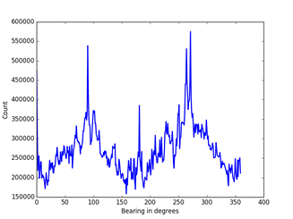
Figure 2: Distribution of aircraft headings in our corpus of 104 million aircraft records.

Since aircraft behave differently in different parts of the world, aggregating data by latitude/longitude bins is necessary to accurately assess unusual aircraft behavior.� Our experiments rounded the latitude and longitude to the nearest integers to define a bin, and this degree of accuracy sufficed for detecting most trends.� We separated the statistics on commercial airlines from those on other aircraft, since commercial airlines are considerably more consistent in their tracks and behavior.� The latitude-longitude-commerciality bins included data for:

The estimated rate of aircraft observed for that bin.� In comparisons between bins, there needs to be an adjustment for the width of a longitude bin as a function of latitude, so .
The average velocity vector in that bin.� Bins along major airlanes will tend to have stronger heading tendencies.� We consider 180 degree deviations to mean the same track, so we compute average the average velocity vector using twice the bearing angle.
The average altitude in that bin.� Bins without major airports will have higher averages.

It is also useful to average in additional bins:

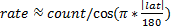
The speed of an aircraft as a function of altitude.� Aircraft closer to the ground are slower (Figure 3).
The count as a function of hour of the day.� Aircraft are less common at night (Figure 4).
The count of the operator (owner) of the aircraft.� Operator-description strings were inconsistent in our corpus, so we regularized them by converting to lower case, removing geographical-origin information, and removing commercial tags such as �inc� and �llc�.
The count of the endpoint pair for the associated track (calculated as discussed in section 4.1).� Routine flights tend to navigate between major airports.
The count of aircraft in bins for great-circle paths.� We use a variant of the Hough transform (Duda and Hart, 1972) that counts evidence for particular great-circle paths.� Great-circle routes can be parameterized by the longitude by which they intersect the equator �and the angle of the intersection from north of .� This can be expressed for a given aircraft position of longitude �and latitude �by the equation �(Karney, 2013).� We can choose a range of integer degree values for �and compute the corresponding values of �in degrees, then increment the position in the two-dimensional array for pair �where �round� is to the nearest integer.

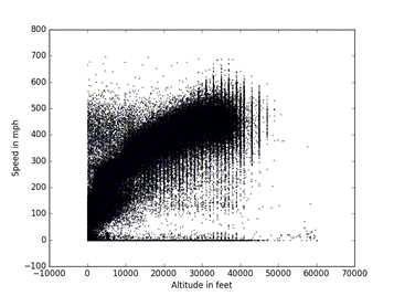
Figure 3: Speed versus altitude for our full corpus.

Figure 4: Count of aircraft records in our corpus as a function of the hour of the day.

4. Ranking aircraft-record anomalousness

Anomalous records of adversary aircraft could indicate planning of military operations or crises.� Other issues indicated by anomalies are safety (Matthews et al, 2014), emergency conditions (DiBernardo and Sleiman, 2016), suspicious following behavior (Cheng et al, 2009), and possible location-surveillance activities (Schmitt et al, 2009).� Note that the anomalous-aircraft problem differs from the more commonly addressed problem with aircraft data, namely classification of platforms into friend, foe, or neutral (Van Gosliga and Jansen, 2003).� Certainly the two problems could interact � an observation of a definite foe with a dangerous track is high priority � but the first problem that must be addressed is whether the data could be potentially interesting, since most air platforms are commercial aircraft flying expected routes.� Our approach is different from that of (Ayhan et al, 2014) in that we must make decisions on priority to reduce data volume, not just provide good visualizations to enable humans to recognize patterns in data.

Figure 5 shows the overall data flow for our ranking scheme for anomalous data.� Several sources of information are compiled into tables, tracks are computed and summarized, and commanders can send their own priorities for ranking.� The result of analysis is two sets of filtered aircraft data, one sent to the command and one sent to sibling platforms.

4.1. Anomalousness clues

There are several kinds of anomalousness.� (Tabassum et al, 2017) labels missing and erroneous records as anomalies (�drop outs� and �missing payloads�) but these are anomalies in data, not in aircraft behavior.� (Das et al, 2011) refers to anomalies found by onboard sensors, but ADS-B does not have access to most of those.� We focused on unusual aircraft flight paths, a type of anomaly that has tactical significance with military aircraft.� From the stored statistics on a training set, we computed degrees of anomalousness for aircraft records on a test set:

� Count: Use the logarithm of the ratio of one plus the number of aircraft observed in the bin to the maximum ever observed in a bin.

� Commerciality: Use the ratio of commercial airline records to total records in the bin. �Anomalousness is this ratio for aircraft not commercial airlines, and one minus this ratio otherwise.

Figure 5: Data flow for the anomaly ranking scheme.

The consistency of the observed heading with the average heading for the latitude-longitude-commerciality bin, measured as the 1 minus the absolute value of the cosine of the angle between them.� Since we store average velocity components at twice the bearing, we also need to take twice the observed heading before comparison, and then use the half-angle formula .
The consistency of the altitude with the averages for the latitude-longitude-commerciality bin.
The consistency of the speed with the altitude of the aircraft.� We obtained a best-fit formula of �using a sample of our data.� Anomalousness is when the ratio of the observed speed to the predicted speed is far from 1, though there were some exceptions for low altitudes during takeoff and landing.

� The logarithm of the ratio of the count of most common aircraft operator of American Airlines and the count of the particular aircraft operator.

� The rarity of aircraft reports at this time of day measured as the logarithm of the ratio of the count in the most common time of day and the count at this time, interpolating within the hour.

� The rarity of aircraft reports on this particular day measured as the logarithm of the ratio of the counts of the busiest day to the count on this day.

� The degree to which the aircraft is not in an airlane as judged by the counts of the great-circle Hough transform described earlier.� For a given latitude-longitude pair, we compute all the nearest corresponding integer-coordinate points it maps to in the space of equator longitude and equator angle of incidence for great circles.

An aircraft can also be considered anomalous if its track considered as a whole is unusual.� We compute tracks by first sorting the data by ICAO number (aircraft code) and then by increasing time.� We then scan the data records for each aircraft to finding starting and ending points for each track, terminating tracks that show no activity for over an hour of time.� Tracks with durations less than 30 minutes were not considered because flights are very rarely this short, and such situations can be due to faulty or disabled transponders.� The one-hour gap heuristic can fail for aircraft on the ground which are still being tracked, generally due to the fault of the pilot in failing to turn off the transponder, and for smaller aircraft that are difficult to track in the air, but it works well for most aircraft.� A pilot may also turn off the transponder too soon once on the ground, meaning the satellite may have insufficient time to pick up its landing location.� This is illustrated by the difference between Figure 6, showing a random sample of all aircraft reports in our sample to the south of San Francisco, California, USA, and Figure 7, showing a random sample of the endpoints of tracks calculated for the same region.� The airlanes are less apparent in the second figure, but can still be traced, indicating tracks starting after leaving an airport or terminating before reaching an airport.� A similar phenomenon of missing data was observed with the North Dakota airport data in (Tabassum, Allen, and Semke, 2017).� It helps that we round track endpoints to the nearest latitude and longitude to define their bins for counting since most of the missing data was within a few miles of airports.

Figure 6: Random sample of aircraft position reports to the southeast of San Francisco (in the upper left).

Figure 7: Random sample of computed track endpoints to the southeast of San Francisco (in the upper left).

Figure 8 shows a typical track profile in altitude.� We compute for each track the starting location and altitude, the destination location and altitude, and the maximum altitude and its associated location.� We also compute the total duration of the track and its average speed, and additional factors for anomalousness:

� The average deviation of the path from a straight path in a two-dimensional projection.� This will be low for commercial flights and possibly high for surveillance and sightseeing flights.

� The average rate of turn of the aircraft over the path for intervals of a minute or more.

� The average altitude difference per unit time.� This will be low for commercial flights and possibly high for military flights and helicopters.

� The average rate of altitude change over the path for intervals of a minute or more.

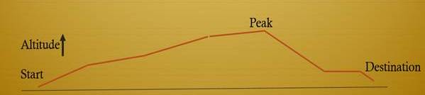
Figure 8: Typical track pattern in altitude.

The pattern of records of a day can also be anomalous even when individual records are not.� This could occur if an adversary were preparing for operations by putting more aircraft or new kinds of aircraft in the air on a day.� It is best to measure aggregate anomalies in latitude-longitude bins because there are wide variations between areas of the world.� We compute three kinds of pattern anomaly factors:

� The atypicality of the count on this day in the latitude/longitude bin from the average count per day in this bin, measured as the absolute value of the logarithm of the counts.

� The histogram in this latitude/longitude bin of aircraft observed on this day compared to the all-day histogram in this bin.� We used a histogram of 32 possible kinds of aircraft distinguished by one of eight areas of the world, military/nonmilitary status, and commercial/noncommercial status.

� The histogram of the speed-altitude mix of aircraft in that latitude/longitude bin observed on this day compared to the all-day histogram in this bin.� Speeds are rounded to the nearest 20 miles per hour and altitudes are rounded to the nearest 2000 feet to create the histograms.

We measured the degree of anomaly of a histogram by one minus the cosine similarity formula; we also tested the Kullback-Leibler divergence but found its results less intuitive.� Table 1 shows example data used for calculation of the second bullet for the bin of latitude 36 and longitude 24.� Listed are the counts over our corpus (12 days total) and those for two particular days.� It can be seen there are significant differences in the number of noncommercial European aircraft and the number of Middle East commercial aircraft, among other things.� The cosine similarity between the overall histogram and September 10 is 0.9765, and between the overall histogram and March 10 is 0.7793, so the day in March is less typical.

4.2. Putting the clues together

To combine the sixteen factors, we used the simplest possible model to test the soundness of our methods, a linear model with equal weights of 1/16.� To ensure that no one factor greatly overwhelmed the others on a particular case, most factors were mapped to a range between 0 and 1 by applying the simplest possible sigmoid function x/(k+x) for some k, with the exceptions of factors which were already in that range.� Table 2 shows the formulas we used.� They were chosen to put average values around 0.25 with a standard deviation of 0.2.� Figure 9 shows the resulting distributions of anomaly values for each factor; time of day has the largest peak due to all the aircraft flying at night.

Table 1: Histograms of aircraft types on two days for an example latitude-longitude bin.

Aircraft registration and type	Total of 10^th day of all 12 months	September 10, 2015	March 10, 2016
North America commercial	31	0	0
South and Central America commercial	5	0	0
Europe commercial	3851	615	201
Africa commercial	144	28	21
Middle East commercial	588	62	212
Central Asia commercial	0	0	0
East Asia and Pacific commercial	0	0	0
North America noncommercial	16	7	1
Other America noncommercial	75	0	5
Europe noncommercial	678	249	2
Africa noncommercial	2	0	0
Middle East noncommercial	13	2	3
Central Asia noncommercial	0	0	0
East Asia and Pacific noncommercial	0	0	0

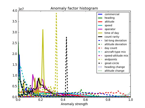
Figure 9: Distribution of the anomaly factors for the aircraft records in our test data.

Table 2: Formulas used for the sigmoid functions on the factors.

Factor	Anomalousness formula
Rarity of aircraft in this lat/long bin	z = difference of natural logarithm of total count and natural logarithm of count in this bin, then a = z / (5+z)
Commercial/noncommercial	a = fraction squared of noncommercial in the lat/long bin for commercial aircraft, fraction squared of commercial in the bin for noncommercial aircraft
Heading atypicality	a = cosine squared of the angle between the aircraft heading and the average heading in this latitude/longitude bin
Altitude atypicality	z is absolute value of difference between altitude (in feet) and average altitude in the bin divided by the standard deviation of the altitude, then a = z / (1+z)
Speed atypicality	z is absolute value of difference between adjusted speed (in miles per hour) and average adjusted speed in the bin divided by the standard deviation of speed in the bin, then a = z / (1+z)
Rarity of aircraft operator	z = logarithm of ratio of count of most common operator and count of this operator, then a = z / (20+z)
Rarity of time of day	z = logarithm of the ratio of count at the most common time of day and count at this time of day (with interpolation), then a = z / (1+z)
Atypicality of count of this day for this lat/long bin	z = absolute value of count on this day minus average count in the lat/long bin, then a = z / (5+z)
Rarity of the best possible airlane match	z = logarithm of the maximum possible airlane count minus the logarithm of the best possible airlane count associated with this latitude and longitude, then a = z / (10+x)
Latitude-longitude deviation from straight path	z = sum of absolute deviations from straight-line path divided by length of straight-line path, then a = z / (1+z)
Altitude deviation from straight up and down	z = logarithm of ratio of total of altitude changes over peak altitude minus start altitude plus peak altitude minus end altitude, then a = z / (0.8+z)
Atypicality of mix of region of origin, government, and commerciality status in bin	a = square root of one minus inner product of histogram for this day with histogram for all days in this bin
Atypicality of mix of altitudes and speeds in bin	a = square root of one minus inner product of histogram for this day with histogram for all days in this bin
Rarity of the track endpoints	z = logarithm of ratio of the maximum endpoint-pair count to the particular endpoint-pair count, a = z / (15+z)
Average rate of heading change	z = heading change per minute, a = z / (100+z)
Average rate of altitude change	Z = altitude change per minute, a = z / (3000+z)

Figure 10 shows the distribution of the evenly weighted sum of the factors for our test corpus of 105 million aircraft records.� The tail on the right represents interesting records; note that the right side of the peak is slightly higher than the left side and likely contains records of nonrandom increased anomalousness that are worth investigating.

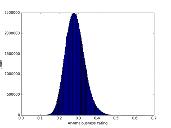
Figure 10: Distribution of overall anomalousness measures for 104 million aircraft records.

Currently we are eliminating 99.7% of the data using our anomaly ranking methods and a threshold of 0.5.� Here are three records from the 0.3% most anomalous.� �Icao� is the aircraft identification number, �trak� is the bearing, and �totaldiff� is the sum of the anomalousness factors.

� icao:"ac49a2", alt:"33000", lat:"35.871804", long:"-111.141494", postime:"1476056189161", spd:"260.0", trak:"184.2", type:"md82", op:"sunrise asset management llc- las vegas", cou:"united states", count-ratio average difference 0:"0.55897", direction average difference 1:"0.6384", altitude average difference 2:"0.18194", adjusted-speed average difference 3:"0.76074", log operator-frequency average difference 4:"0.2355", hour average anomaly 5:"0.2244", count rarity 6:"0.26813", latlong deviation 7:"0.27621", altitude deviation 8:"0.58646", day count deviation 9:"0.75491", day type-mix deviation 10:"0.85054", day altspeed-mix deviation 11:"0.91162", endpoint rarity 12:"0.33685",great circle rarity 13: �0.07029�, totaldiff:"0.50651"

� icao:"43e821", alt:"41000", lat:"40.915786", long:"-70.65189", postime:"1476057229821", spd:"547.4", trak:"77.2", type:"gl5t", op:"jasmin aviation ltd", cou:"isle of man", count-ratio average difference 0:"0.43547", direction average difference 1:"0.00157", altitude average difference 2:"0.56511", adjusted-speed average difference 3:"0.49604", log operator-frequency average difference 4:"0.37589", hour average anomaly 5:"0.22349", count rarity 6:"0.2473", latlong deviation 7:"0.50664", altitude deviation 8:"0.55542", day count deviation 9:"0.90831", day type-mix deviation 10:"0.99207", day altspeed-mix deviation 11:"0.89144", endpoint rarity 12:"0.33685", great circle rarity 13:�0.12844�totaldiff:"0.50274"

� icao:"a57140", alt:"9200", lat:"46.546326", long:"-93.637747", postime:"1489099087672", spd:"183.0", trak:"69.9", type:"ac95", op:"united states department of commerce�� - mcadill afb", cou:"united states", count-ratio average difference 0:"0.51246", direction average difference 1:"0.4216", altitude average difference 2:"0.53588", adjusted-speed average difference 3:"0.5424", log operator-frequency average difference 4:"0.36397", hour average anomaly 5:"0.14728", count rarity 6:"0.34395", latlong deviation 7:"0.28742", altitude deviation 8:"0.59401", day count deviation 9:"0.64431", day type-mix deviation 10:"0.87565", day altspeed-mix deviation 11:"0.9882", endpoint rarity 12:"0.33685", great-circle rarity 13:"0.42515", totaldiff:"0.50137"

Figure 11 shows the first two principal components of a random sample of the anomaly data for the 5% most anomalous records.� Clustering is definitely apparent in the middle and upper left.

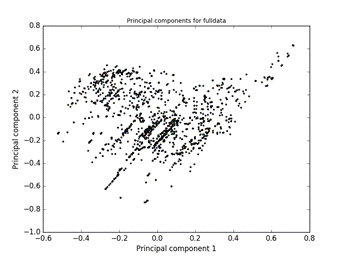
Figure 11: First two principal components of a random sample of the anomaly data.

4.3. �Outlier visualization

To analyze the most anomalous records we find by our rating scheme, it is helpful to do visualizations of particular attributes in the data.� To do this it is helpful to take random samples; a size of 5000 was reasonable for a useful display. �Figure 12 shows the distribution of peak values versus longitude in a sample, showing that high altitudes tend to occur over centers of continents.� Similarly, Figure 13 shows the distribution of average relative track speeds versus longitude, showing the high speeds also tend to occur over centers of continents.� This suggests that atypicality of peak and speed can be fit to a longitude curve.

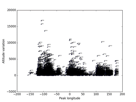
Figure 12: Altitude variation versus peak longitude for a random sample of 5000 tracks.

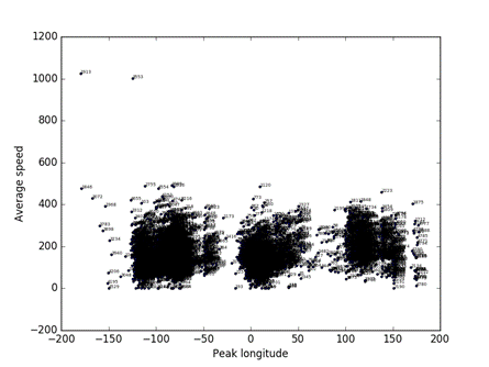
Figure 13: Average speed versus peak longitude for a random sample of 5000 tracks.

Figure 14 shows the relationship between track duration and peak altitude of the track.� Clearly longer tracks can go higher, but there are also plenty of short flights.� Figure 15 shows a counterintuitive relationship between track duration and average speed, where longer flights have shorter speeds; this may be due to longer flights being larger aircraft that have more records on the ground.� Finally, Figure 16 shows the relationship of the two deviations, straight-line deviation and altitude variation.� Vehicles on the ground are creating a number of spurious points on the right, and many commercial aircraft are going up and down without deviating from straight-line paths, but we need to investigate the lower left part of the graph at a finer grain of resolution.

Figure 14: Track duration versus peak altitude for a random sample of 5000 tracks.

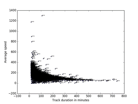
Figure 15: Average speed versus duration for our corpus.

Figure 16: Altitude deviation versus straight-path latitude-longitude deviation for a random sample of 5000 tracks.

4.4. Clustering to find anomalies

We studied several kinds of automated clustering to enable automated extraction of the above kinds of outliers in tracks.� The attribute sets we used for clustering are summarized in Table 3.� Weights on the attributes were important in computing distances when the attributes were not commensurate.� The standard deviation of the attribute was a useful guide.� For instance, longitude had 2.5 more standard deviation than latitude due to the high-latitude tracks in the Northern hemisphere, so we multiplied longitudes by 0.4 before computing distances.

We used our test set to find cluster centers using the K-Means algorithm, then clustered the full data using those centers.� The computation time of K-Means is proportional to the number of data items times the number of clusters times the number of iterations to reach convergence, so it can take considerable time on a large data set.� We thus ran K-Means on our sample of the data (110 million records), and used the cluster centers it found for larger sets of data.� We tested a larger set as described in the next section.

The total number of tracks was 776,014.� The last column of Table 3 gives the number of tracks that more than three times beyond the average radius of their assigned cluster for the given clustering scheme with the test set.� This provides an alternative way to define anomalies that may find different kinds than our previous approach.

Table 3: Attributes used for clustering experiments.

Tag	Attributes	Weights	Phenomena addressed by clusters	Number of anomalous tracks
Latlong	Start latitude, start longitude, end latitude, end longitude	1, 0.4, 1, 0.4	Scheduled airline city pairs	2398 (0.3%)
Latlong2	Start latitude, start longitude, altitude-peak latitude, altitude-peak longitude, end latitude, end longitude	1, 0.4, 1, 0.4, 1, 0.4	Scheduled airline flights	2816 (0.4%)
Altprofile	Start altitude, peak altitude, end altitude	1, 1, 1	Commercial versus noncommercial aircraft	1183 (0.2%)
Startdur	Start latitude, start longitude, track duration	1, 0.4, 0.08	Major commercial airports	677 (0.1%)
Deviations	Track duration, latitude-longitude deviation, altitude deviation	0.005, 0.2, 1	Regularity of tracks	709 (0.1%)

5. Analyzing ship data for anomalies

We also had 5.96 million records of ship data from a previous project involving the South China Sea.� We applied our aircraft methods to this data to see how well they generalized.

The ship data came from AIS systems installed on ships (see www.marinetraffic.com), and included these fields:

� ship name: Not used except for debugging

� MMSI ship-identification number: analogous to the ICAO number for aircraft

� IMO ship code: not used

� Vessel type: used for deciding commercial/noncommercial analogously to aircraft

� Latitude and longitude: used

� Speed in knots: used

� Heading in degrees: used

� Timestamp: used

We excluded a number of records with speeds that were null or over 100 knots.� We noticed that ship positions became less accurate the further they were from shore, so this needs to be accounted for in the anomaly calculation.

We created bins similarly to aircraft data to create latitude-longitude-commerciality count, average heading, speed count, hour-of-day count, and latitude-longitude-day count.� Ships do not have the freedom of travel that aircraft do, and were restricted to a limited set of latitude-longitude bins.� Tracks were partition at gaps of at least 1000 hours or 41.7 days in the reporting of positions.� We also needed to remove all references to altitudes.� The anomaly factors we computed were:

� Commerciality atypicality

� Heading atypicality

� Speed atypicality

� Ship-type atypicality

� Hour-of-day atypicality

� Count atypicality for its latitude-longitude-commerciality bin

� Track deviation from straight line

� Day count atypicality for its latitude-longitude bin

Figure 17 shows the distribution of the anomaly factors computed on the ship data.� These look quite reasonable.

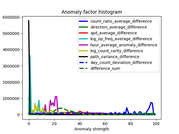
Figure 17: Anomaly factors for the ship data.

6. Big-data implementations

Initial experiments on 12 days of data (13.6 million records) took 0.9 hours per day of data to process.� Our goal is to handle a year�s worth of data for an adequate demonstration of capability, which means files in the terabyte range and disk-intensive input/output.� So distributed processing appears necessary (Zhou, 2018).� Eventually we expect that this processing will be done on the aircraft collecting the initial sensor data where filtering of data will do the most good in reducing bandwidths.� Multiprocessor architectures are decreasing in price and it reasonable to consider they could be put on aircraft.

6.1. Hadoop-Spark implementation

One set of experiments used the distributed processing architecture of the Hadoop Distributed File System HDFS (http://hadoop.apache.org/hdfs) with which a divide-and-conquer approach can parallel-process the data on individual nodes and then aggregate the results.� HDFS also provides a programming paradigm MapReduce whereby programmers can specify the code for the Map and the Reduce phase, and input/output the data in key-value pair format, and let HDFS handle the rest.� To reduce disk input/output, the SPARK2 software for using HDFS is more memory-centric than traditional compilers. HDFS is built on commodity hardware with open-source software, and has lesser costs than most high-performance computing.� Its community develops software and tools, and the data size makes HDFS a cost-effective fit for processing ADS-B files.� We confirmed further speed improvements to HDFS when using Infiniband network cards for a larger bandwidth pipe and using solid-state drives in some server nodes without overly increasing the costs. �However, there were challenges in moving the data to HDFS and adapting our programs to the SPARK2 environment.

The steps in our processing posed different kinds of challenges for a Hadoop/HDFS/SPARK2 implementation:

� Initial data filtering was easily split and merged since filtering can be by individual records.

� Calculation of average bin values was easily split and merged by keeping counts and totals separately.

� Track calculation needed some care in design.� Splitting needs to be by aircraft, keeping its data together on a single processor, and this requires first sorting the data by aircraft, then calculating minima, maxima, and averages for subtables.

� Calculation of anomalousness adapted quite well to the new design, but was time-consuming to implement because of the many calculations involved.� It needs to be done for each aircraft on the same processor that holds the track data and binned data for the same area as the main data records, so planning is necessary to keep the necessary data together.

Tests we conducted used an Apache Spark (�a unified analytics engine�) implementation of distributed processing on three Hadoop server machines (Intel Xeon-5s with 384GiB memory and 8, 8, and 12 cores respectively) with a database-oriented programming package.� Spark has been used with analysis of ship positions (Liu, 2018).� Our tests have not been completed.� Nonetheless, Table 3 below shows the promising results so far compared to a control single-processor Python implementation.� It can be seen that all but the fourth method had speedups beyond the increase in the number of cores, which we infer is due to the effective use of graphical processing units (GPUs) on these machines.� However, the track analysis did not show as much a speedup since it required sorting as well.

Table 4: Results of distributed-processing experiments.

Process	Time for single processor on the Spark site	Time for Hadoop Spark implementation	Time per record for Spark implementation
Move data from database to files	612 minutes	26.6 minutes	0.00117353
Count aircraft in lat-long bins	70.6 minutes	2.5 minutes	0.00011029
Average the speed in altitude bins	72.7 minutes	1.0 minutes	0.00004412
Summarize the aircraft tracks	59.5 minutes	22.3 minutes	0.00098382
Find anomalies using the first 7 factors	211.2 minutes	18.5 minutes	0.00081617

6.2. Supercomputer-Spark experiments

We also conducted experiments with our code in Apache Hadoop and the tool Gradle on the NPS Hamming/Grace supercomputer cluster with over 3000 cores.� More details are given in the Appendix.� We used the Gradle tool and stored some of the intermediate results in the Parquet format.� We took a different sample of the aircraft data of 1.531 billion records, more than 100 times the size of the previous experiments.� Timing results are shown in Table 5.

Table 5: Results of distributed processing of aircraft data �on the Hamming / Grace supercomputer cluster.

Aircraft-data Process	Total time for Hadoop/Gradle on supercomputer	Time per record
Set up processing	33.25 minutes	0.00000130
Aggregate the data	9.60 minutes	0.00000038
Find anomalies using the first 10 aircraft factors	10.27 minutes	0.00000040
Assign clusters based on cluster centers found previously in uniprocessor implementation	112.87 minutes	0.00000442
Create graphs of anomaly analysis (optional)	53.18 minutes	0.00000208

We also tested this approach on the smaller amount of ship data, as summarized in Table 6.� Times per record are increased due to the increased influence of time to transfer data to and from processors.

Table 6: Results of distributed processing of ship data on the Hamming / Grace supercomputer cluster.

Ship-data Process	Total time for Hadoop/Gradle on supercomputer	Time per record
Set up processing	1.73 minutes	0.00001745
Aggregate the data	1.62 minutes	0.00001628
Find anomalies using the 10 ship factors	1.87 minutes	0.00003893
Assign clusters based on cluster centers found previously in uniprocessor implementation, plus create graphs of anomaly analysis	14.45 minutes	0.00014547

These are impressive speeds.� This kind of supercomputer could be installed in a shore base.� However, it would be expensive and is too big to put on an aircraft, and obtaining sufficient power could be a limitation for installing it on a Navy ship.

7. Conclusions

Anomalies against a background of routine activities are key clues to human intentionality.� With the capability to collect huge amounts of data today, we need a strategy to find anomalies without requiring huge processing times.� We have shown that this can be done for basic aircraft tracking data by choosing useful factors carefully, and filtering and summarizing the data in an intelligent and efficient way.� This can provide early warning about adversary plans.

As for future work, group anomalousness can also measure interactions between aircraft.� A key goal of air-traffic control is to monitor for possible collisions between aircraft, and near approaches can be important in a military setting too.� (Chen et al, 2014) offers a number of useful ideas for monitoring land vehicles which could be applied to airspaces.� For instance, a vehicle approaching another vehicle usually slows down; when it does not, it is anomalous.� This approach can also be applied to other kinds of sensor data.�

A nonlinear neural network could be a good way to generalize our linear model.� The analysis we have done so far suggests that a mere 16 factors could provide good performance as the input to such a network rather than using the raw data or a convolutional neural network.� One issue is that we actually need an unsupervised learning model, and neural networks are much better suited for supervised learning.� However, autoencoding can be done with neural networks as an unsupervised process.�

Acknowledgements

This project was supported by the Naval Research Program at the Naval Postgraduate School under JONs W7B26 and W7A99 and topics NPS17-N185-B and NPS18-0193-B.� The views expressed are those of the authors and do not represent the U.S. Government.

References

Ayhan, S., Fruin, B., Yang, F., and Ball, M., NormSTAD Flight Analysis: Visualizing Air Traffic Patterns over the United States.� Proc. Of the 7^th ACM SIGSPATIAL International Workshop on Computational Transportation Science, November 2014.

Chen, Q, Qiu, Q., Wu, Q., Bishop, M., and Barnell, M., A Confabulation Model for Abnormal Vehicle Events Detection in Wide-Area Traffic Monitoring.� IEEE Intl. Inter-Disciplinary Conf. on Cognitive Methods in Situation Awareness and Decision Support, 2014.

Cheng, K., Tumbokon, F., Sahu, R., Bao, J., and Beling, P., Track Based Characterization of Vehicle Behavior, Proc. Systems and Information Engineering Design Symposium, Charlottesville, VA, April 2009, pp. 269-274.

Das, S., Mathews, B., and Lawrence, R., Fleet Level Anomaly Detection of Aviation Safety Data.� Proc. IEEE Conf. on Prognostics and Health Management, Montreal, Canada, 2011.

DiBernardo, G., and Sleiman, S., P6 � Cause for Emergency.� Proc. Large Scale Data Engineering, 2016.� Retrieved from https://event.cwi.nl/lsde/2016/papers/group11.pdf, March 11, 2018.

Duda, R., and Hart, P., Use of the Hough Transformation to Detect Lines and Curves in Pictures.� Communications of the ACM, Vol. 15, January 1972, pp. 11�15.

Federal Aviation Administration, Automatic Dependent Surveillance-Broadcast (ADS-B).� Retrieved February 13, 2018 from https://www.faa.gov/nextgen/programs/adsb.

Forer, S., and Yliniemi, L., Monopolies Can Exist in Unmanned Airspace, Proc. Of the Genetic and Evolutionary Computation Conference, July 2017.

Karney, C., Algorithms for Geodesics.� Journal of Geodesy, Vol. 83, 2013, pp. 43-55.

Liu, B., Parallel Maritime Traffic Clustering Based on Apache Spark.� Retrieved from pdfs.semanticscholar.org/ee57/da09d549d6d074de29bf03aa2b33948295ad.pdf, 2018.

Matthews, B., Nielsen, D., Schade, J., Chan, K., and Kiniry, M., Automated Discovery of Flight Track Anomalies.� Proc. 33rd IEEE/AIAA Digital Avionics Systems Conf., Colorado Springs, CO, US, October 2014, pp. 4B3-1-4B3-14.

Rowe, N., Reed, A., Schwamm, R., Cho, J., Flores, J., and Das, A.� Networks of Simple Sensors for Detecting Emplacement of Improvised Explosive Devices.� Chapter 16 in F. Flammini (Ed.), Critical Infrastructure Protection, WIT Press, 2012, pp. 241-254.

Salcido, R., Kendall, A., and Zhao, Y., Analysis of Automatic Dependent Surveillance-Broadcast Data.� Proc. Deep Models and Artificial Intelligence for Military Applications, AAAI Technical Report FS-17-03, 2017.

Schmitt, D., Kurkowski, S., and Mendehall, M., Automated Casing Event Detection in Persistent Video Surveillance, Proc. Intl. Conf. in Intelligence and Security Informatics, Richardson, TX, US, June 2009, pp. 143-148.

Tabassum, A., Allen, N., and Semke, W., ADS-B Message Contents Evaluation and Breakdown of Anomalies.� IEEE/AIAA 36^th Digital Avionics Systems Conference, 2017.

U.S. Navy SPAWAR Enterprise Architecture Data Strategy Working Group, Overarching Concepts, slides dated March 10, 2016.

US DoD Director of Defense Research and Engineering, Joint Warfighter Science & Technology Plan, February 1998.

Van Gosliga, S., and Jansen, H. (2003).� A Bayesian Network for Combat Identification.� Proc. NATO RTO IST Symposium on Military Data and Information Fusion, Prague, CZ, October, NATO RTO-MP-IST-040.

Zhou, J., Using Apache Spark to Analyze ADS-B Data with Machine-Learning Techniques.� M.S. thesis, U.S. Naval Postgraduate School, June 2018.