ABSTRACT

Drives found during investigations often have useful information in the form of email addresses which can be acquired by search in the raw drive data independent of the file system. Using this data we can build a picture of the social networks that a drive owner participated in, even perhaps better than investigating their online profiles maintained by social-networking services because drives contain much data that users have not approved for public display. However, many addresses found on drives are not forensically interesting, such as sales and support links. We developed a program to filter these out using a Naïve Bayes classifier and eliminated 73.3% of the addresses from a representative corpus. We show that the byte-offset proximity of the remaining addresses found on a drive, their word similarity, and their number of co-occurrences over a corpus are good measures of association of addresses, and we built graphs using this data of the interconnections both between addresses and between drives. Results provided several new insights into our test data.

Keywords: digital forensics, electronic mail, email, addresses, users, filtering, networks, visualization

This paper appeared in the Proceedings of the Eighth International Conference on Digital Forensics and Computer Crime, New York, NY, September 2016, as well as the Journal of Digital Forensics, Security, and Law, Volume 11, No. 2.

1. Introduction

Finding social networks is important in investigating organized crime and terrorism. Social networks can be learned from connections recorded by social-networking services and discussion-forum Web pages. However, this is public information, and is often of limited value in a criminal investigation in which subjects conceal key information about their contacts. Furthermore, license agreements often prohibit automated analysis of such data without permission, and much user data may not be accessible without the cooperation of the service or page owner. A better source could be the contacts users store on their computers and devices in the form of electronic-mail (email) addresses, telephone numbers, street addresses, and personal names. Some may be information of which users are not aware because it was stored by software or left in unallocated space after deletions.

This work focuses on email-address data. Such data can indicate personal connections by the nearby placement of pairs of addresses on a drive, similarity of words in address pairs suggesting aliases, or repeated association of address pairs on a set of drives. We may thus be able to infer networks of contacts of varying connection strengths from the data on one drive alone. We can then use several methods to build visualizations of the networks to make them easier to understand. A key obstacle is that many addresses on a drive are uninteresting because businesses and organizations put contact addresses into their Web pages and software, so we must first exclude these. Note that seeking addresses on drives has advantages over inspecting the records of a mail server because it can find older addresses removed from a server or potential contacts never used to send mail.

2. Literature review

Most work on visualizing social networks has focused on social-networking sites where links between people are made explicit through a variety of friend and contact links (Holzer, Malin, and Sweeney, 2005; Zhou et al, 2006; Polakis et al, 2010). They can also be extracted from text by nearby mentions of names of people (Laclavik et al., 2012) though nearness may be coincidental. So far there has been little attention to the mining of addresses from drives, their classification, or their connection to social networks. There has been work on the classification of email messages from their message headers (Lee, Shishibori, and Ando, 2007) but headers provide significantly richer contextual information than lists of email addresses found scattered over a drive.

3. Test Setup

This work primarily used the Real Data Corpus (Garfinkel et al, 2009), a collection of currently 2401 drives from 36 countries after excluding 961 empty or unreadable drives. These drives were purchased as used equipment and represent a range of business, government, and home users. We ran the Bulk Extractor tool (Bulk Extractor, 2013) to extract all email addresses, their offsets on the drive, and their preceding and following characters. Email addresses consist of a username of up to 64 characters, a "@", and a set of domain and subdomain names delimited by periods. Bulk Extractor bypasses the file system and searches the raw drive bytes for patterns appearing to be email addresses, so it can find addresses in deleted files and slack space. On our corpus this resulted in 292,347,920 addresses having an average of 28.4 characters per address, of which there were 17,544,550 distinct addresses. The number of files on these drives was 61,365,153, so addresses were relatively infrequent, though they were more common for mobile devices.

Sample output of Bulk Extractor:

65484431478 ttfaculty@cs.nps.navy.mil vy.mil>\x0A> To: "'ttfaculty@cs

69257847997 info@valicert.com 0\x1E\x06\x09*\x86H\x86\xF7\x0D\x01\x09\x01\x16\x11info@valicert.com\x00\x00\x00\x00\x00\x00\x00\x00\x00\x00\x00\x00\x00\x00\x00\x00

Bulk Extractor's email-address scanner seeks domain/subdomain lists containing at least one period and punctuating delimiters in front and behind the address. Currently Bulk Extractor handles common compressed formats but cannot recognize non-Ascii addresses. Recent standards for international email in the IETF's RFC 6530 allow the full Unicode character set in both usernames and domains (Klensin and Ko, 2012) so that must be considered in the future. Most of our corpus predates the standard.

This work primarily used an "email stoplist" provided by the U.S. National Institute of Standards and Technology (NIST) by running Bulk Extractor on a portion of their software collection. Email addresses found inside software are likely software contact information and unlikely to be interesting, but this is not guaranteed because software developers may have inadvertently left personal addresses, or deliberately put them in to enable unauthorized data leakage. We supplemented this list with three other sources: known "blackhole" addresses used for forwarding spam (gist.github.adamloving/4401361, 482 items), known scam email addresses (www.sistersofspam.co.uk, 2030 items), and addresses found by us using Bulk Extractor on fresh installs of standard Windows and Macintosh operating systems (332 items). After eliminating duplicates, the stoplist had 496,301 addresses total.

We also created four important word lists for use in interpreting the words within addresses:

· 809,858 words of the online dictionaries used in (Rowe, Schwamm, and Garfinkel 2013). The English word list was 223,525 words from two dictionary sources and included morphological variants. 587,258 additional words were from Croatian, Czech, Dutch, Finnish, French, German, Greek, Hungarian, Italian, Norwegian, Polish, Portuguese, Romanian, Serbian, Spanish, Swedish, and Turkish dictionaries and transliterated to Ascii. We did not consider languages like Arabic and Chinese whose transliteration to Ascii was problematic. We converted words to lower case, eliminated those that were also personal names and generic usernames, and eliminated non-English one-letter and two-letter words since they caused too many false matches to code strings. Unlike in our previous work, we did not include abbreviations, acronyms, and words found only inside software.

· 102,426 personal names including both given names and surnames. We obtained international coverage by using a variety of resources including proposed baby names. Another approximately 15,000 were found by inspecting the training set and stop list.

· 3,515 names of email and messaging servers. Some had words like "mail" and "chat" in their domains, but others required Web research to determine their function.

· 2,813 "generic usernames" representing generic addresses such as business contacts. These we identified by manually inspecting the training set and stoplist. Table 1 gives examples.

Table 1: Example generic usernames.

auctions	backup	beauty
callcenter	conference	download
editor	feedback	group
homepage	ideas	jobsindia
linux	marketinfo	nobody
outlet	passwords	registration
response	save	testing
tickets	update	yourmatches

4. Eliminating Uninteresting Addresses

A first step is to remove addresses unlikely to be interesting in a forensic investigation. We have clues in both the username and the domain/subdomain names. For instance, johnsmith@friendlymail.co.uk uses two human names in the username, and a domain name that includes "mail" to suggest a mail server; these clues suggest it is an interesting address. On the other hand, direct-sales@auction.treasures.com uses the frequent generic term "sales" in the username, and the domain is a ".com" without indication of a server; so mail to or from this address is unlikely to be interesting, and the address should be removed from further analysis. Case usually does not matter in addresses, so we converted all to lower case after the case analysis described in section 4.4.

4.1. Training/test sets

We obtained data for training and testing our user-address identification by first taking a random sample of 6638 of the 17 million distinct addresses in our corpus, manually inspecting them to assess whether they were likely to be personal user addresses, and labeling them accordingly. Most were easy to assess, but some required research on the Web to determine the nature of their sites. A few cases in the random sample (about 50 or so) about which we could not reach a clear determination were excluded. We needed to exclude these because it is not ethical to just try sending mail to an address, and many addresses are no longer valid since our corpus spans twenty years. We supplemented this random sample with a random sample of 1000 items from the NIST address stoplist, marking them as nonusers. This resulted in 7638 distinct addresses of which 3061 were labeled as users and 4577 were labeled as nonusers. We used this test for both training and testing, choosing disjoint subsets from it.

4.2. Clues to interesting and uninteresting addresses

The stoplist matched 27.5% of the addresses in our corpus, and missed many obviously nonuser addresses. Thus it was important to use evidence from multiple other clues for the remaining addresses. We compiled a set of clues from a number of sources for testing:

· Whether the address was in our combined stoplist.

· The number of drives on which the address occurred in our corpus. Addresses that occur on many drives are likely to be contact addresses of software vendors, which we consider uninteresting. (That reflects the random-sample nature of our corpus; in other corpori, addresses occurring on many drives may well be interesting.) Note that it is important to count the number of drives rather than the number of occurrences of the address because addresses can occur repeatedly on a drive when it is used for automatic contact. Figure 1 shows the distribution of the logarithm of the number of drives on which an address occurred, ignoring the approximately 14 million addresses that occur on only one drive so the leftmost bar is for 2 drives.

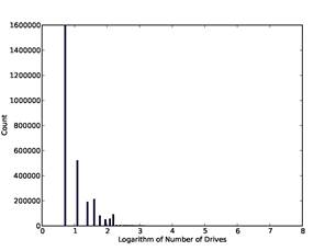
Figure 1: Histogram of number of drives on which an email address occurs in the full corpus, versus the natural logarithm of the number of drives.

· The occurrence of automatic-contact patterns in the characters preceding the address. Table 2 shows the patterns we used, found by analysis of our training sets.

· The number of times in succession the address occurred on the drive without intervening addresses; repeated occurrences suggest automated logging. Figure 2 plots the fraction of user addresses as a function of the natural logarithm of successive occurrences, for the addresses of the training set using counts from our full corpus. From this we chose a threshold of 3.91 (50 occurrences) for a boolean clue.

· The length in characters of the domains and subdomains.

· The domain type. The categories we used were mail or messaging server, one of {.com, .co, .biz, .coop}, one of {.edu, .ac, .pro}, one of {.org, .gov, .govt, .gv, .gouv, .gob, .mil, .int, .museum, .arpa}, one of {.net, .info, .aero}, and any other domain. Mail and messaging servers were defined by occurrence of a known server name in any of the words delimited by periods following the "@" or any inclusion of the string "mail". The other domain categories were defined by the subdomain on the right end after removing any two-letter country codes. This means that "yahoo.com" was considered a server but "legalsoftware.co.uk" was considered a ".com".

Table 2: Patterns we seek in immediately previous characters to indicate automated-contact addresses.

" for <"	"> from:"
">from: cab <"	"return-path: <"
"internet:"	"email="
"mailto:"	"fromid="
"set sender to"	"email address:"
"/Cookies/"

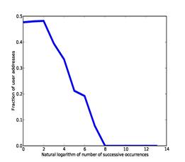
Figure 2: Fraction of user addresses versus the natural logarithm of the number of times they occurred in succession in our training set.

· The type of country in the domain name (assuming U.S. if none). The categories we used were U.S., developed world, developing world, and other.

· Whether a word in the domain-subdomain list matched a word in the username, e.g. "bigcorp.sales@bigcorp.sphinx.ru".

· The length in characters of the username.

· Whether the first character of the username was a digit.

· Whether the last character of the username was a digit.

· The assessed likelihood of the username being a human name once split as necessary into recognizable components, as will be explained in section 4.4.

· The type of file, if any, in which the email address occurred based on its extension and directory. This requires running a different tool to calculate offset ranges of files (we used the Fiwalk tool in SleuthKit), and matching address offsets to these ranges. Only 1673 of the 7638 addresses in our training set occurred even once within a file, so we ignored this clue in tests although it may help on occasion.

4.3. Evidence combination

To combine clues in these experiments, we used Naïve Bayes inference in the odds form:

Here U represents the identification as a user address, represents the occurrence of the ith clue, o means odds, and "|" means "given". Linear weighted sums such as with artificial neural networks and support vectors are a mathematically similar alternative related logarithmically to the above formula. Decision trees are not appropriate for this task because few of the clues are binary, and case-based reasoning is not appropriate because it could require considerable computation time to find the nearest match for this task which includes many nonnumeric attributes. We did not use any weighting on the clues other than that provided by the computed odds themselves, an approach to weighting which we have found sufficient in previous experiments.

To smooth for clues with low counts, we included the Laplacian addition constant :

where means the count of X, and ~X means not X. In the experiments we will discuss with 100 random runs with the same random seed before each group of 100, we calculated the F-score when varying the constant as shown in Table 3. (F-score is defined as the reciprocal of 1 plus the ratio of the total of false positives and false negatives to twice the total of true positives.) So it appeared that a constant of 1 was sufficient, and we used that in the experiments described below. We could not use 0 because random subsets might miss the clues.

4.4. Handling difficult clues

Several clues are numeric and we must map the numbers to probabilities. For example, Figure 3 plots the fraction of user addresses in the training

Table 3: Results on varying the additive constant in the odds calculation.

	Best F-score
1	0.94659
3	0.94587
10	0.94284
100	0.94086

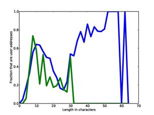
Figure 3: Fraction of user addresses as function of length of username (blue) and length of domains (green) for our training set.

set as a function of length of the username (blue curve with larger input range) and length of the domain and subdomains (green), averaging each adjacent pair of lengths. The dip in the middle of the username curve is interesting; to the left are usernames that are short enough for users to comfortably type themselves, to the right are automated reporting addresses about users sent by software, and in between are lengths too long for users but too short for automated reporting. Note there are username lengths right up to the SMTP-protocol maximum of 64 characters. To model this data, we split the username lengths into four ranges (at 8, 15, and 30) and domain-name lengths into three ranges (at 8 and 15).

Recognizable words in the username are a good clue as to the nature of an address. Generic usernames are a strong negative clue to user addresses, matches to personal names are a strong positive clue, and matches to other human-language words are somewhere in between. After some careful analysis confirmed by subsequent results, we assigned -6, +6, and -2 to these respectively.

If the whole username was not recognized as a word, we tried segmenting it to find recognizable pieces. We segmented at any punctuation mark, any transition from lower to upper case, and any transition between characters and digits. We also segmented username pieces not in our wordlists into two or three pieces that we could recognize, e.g. "joedonsmith" into "joe", "don", and "smith". To find such splits we started with even splits and progressively considered more uneven splits until we found something that we recognized for all the parts, requiring pieces to be at least three characters. We also allowed for one or two letters on the front or end, e.g. "rksmith".

When we could partition a username into multiple pieces, we averaged the weights of pieces of three characters or more and rounded to the nearest integer. This gave 13 possible values ranging from -6 to +6. If we did not recognize a piece after trying all possible splittings, we assigned it a weight of 0. So for example, the username "littlesuzyb_personal" has "personal" for -2, then "littlesuzyb" contains "little" for -2 and "suzyb" can be split into "suzy" and "b" for +6 ("b" has no weight), for an average of 2/3 which rounds to +1.

4.5. Results

We did cross-validation of clues by using a randomly selected 80% of the training set for training and 20% for testing. Table 4 and Table 5 show the mean odds computed for each of the clues in 100 runs, selecting a different training and test set each time from the pool of 7638, plus a standard deviation over the runs. The best F-score for separation of users from nonusers was obtained at a threshold of 0.3916. Prior odds for these runs (the odds of a true user) were 0.8872 with a standard deviation of 0.0102. It can be seen that the weights in the range -6 to +6 on the username words are mostly consistent with odds, which is why we chose the weights that we did. Ratings of +4 and +5 were rare and gave inflated odds values.

Another test for clue redundancy is to remove each clue in turn and see if it hurts performance measured by the F-score. Table 6 shows the results. Of these clues, the successive-occurrences, first-digit, and number-of-drives clues appear to be

Table 4: Odds of a user address given various general and domain clues based on the training set.

Mean odds	Standard deviation	Description
0.001	0.00001	Address in stoplist
1.301	0.0158	Address not in stoplist
0.0688	0.0094	Software-suggesting preceding characters
0.8910	0.0102	No software-suggesting preceding characters
1.0669	0.0128	Occurs only on one drive
0.4563	0.0228	Two drives
0.1518	0.0115	3-10 drives
0.0056	0.0002	>10 drives
0.9053	0.0113	Occurs 10 times or less in succession
0.2348	0.0274	Occurs more than 10 times in succession
0.3741	0.0145	Domains length < 8
1.2228	0.0156	Domains length 8-15
0.3406	0.0105	Domains length > 15
5.0111	0.0948	Server name in domains
0.0148	0.0013	.com domain
0.2586	0.0182	.edu domain
0.0085	0.0019	.org domain
0.3251	0.0268	.net domain
0.0293	0.0032	Other domain
0.0383	0.0087	Username word matches domain words
0.8898	0.0103	Username word does not match domain words
1.0246	0.0141	U.S. domain
0.3844	0.0120	Developed non-U.S. world domain
3.6160	0.1447	Developing world domain
0.3756	0.0165	Rest of the world domain

redundant. We excluded the latter from further analysis; kept the first when it showed better in the full corpus; and kept the third clue because the rare occurrence of multiple drives for addresses in the training set made this an unfair test.

Figure 4 shows the overall histogram of address ratings for the corpus. The blue curve is our full corpus, and the green curve is for our stoplist with counts multiplied by 5 for easier comparison (with the stop-list match clue omitted in calculating the

Table 5: Odds of a user address given various username clues based on the training set.

Mean odds	Standard deviation	Description
0.2453	0.0057	Username < 8 characters
1.3546	0.0209	Username 8-15 characters
0.8023	0.0263	Username 16-29 characters
3.5833	0.169	Username > 29 characters
0.8858	0.0354	First username character is digit
0.8874	0.0110	First username character is not a digit
2.1489	0.0560	Last username character is digit
0.6931	0.0088	Last username character is not a digit
0.0377	0.0053	Username weight -6
0.0744	0.0084	Username weight -5
0.2754	0.0316	Username weight -4
0.2171	0.0272	Username weight -3
0.6291	0.0235	Username weight -2
0.7464	0.0587	Username weight -1
0.6352	0.0167	Username weight 0
1.5080	0.1253	Username weight 1
1.4634	0.0530	Username weight 2
1.7459	0.0978	Username weight 3
5.6721	0.6841	Username weight 4
16.400	1.6673	Username weight 5
1.1881	0.0208	Username weight 6

rating). There are peaks at both ends of the blue curve, so most addresses appear unambiguous to the rater. Note that the stoplist had a few highly-rated addresses like "john_smith@hotmail.com" which were uninteresting software contacts but provide no obvious clue. By setting the threshold to 0.3916, the average of those for the best F-scores on the training set, we identified 78,029,211 address references as user-related, 26.7% of the total.

Table 6: Effects on performance of removing each clue in turn in analyzing the training set.

Clue removed	Best F-score
None	0.9433
Address in stoplist	0.9244
Software-suggesting previous characters	0.9430
Number of drives on which it occurs	0.9436
Number of occurrences in succession	0.9433
Length of domains in characters	0.9411
Domain type	0.7810
Type of country of origin	0.9335
Match between domain and username	0.9416
Length of username in characters	0.9330
Whether first character is digit	0.9433
Whether last character is digit	0.9334
Username weight	0.9287

Figure 5 plots precision versus recall for our training set. (Recall is the fraction of user addresses above the threshold of all those manually identified as user addresses; precision is the fraction of user addresses above the threshold of all those above the threshold.) It can be seen that many addresses are unambiguously nonusers, but there were a small number of difficult cases. Thus the precision, while generally greater than 0.95, improves only gradually with increasing threshold whereas recall improves quickly with decreasing threshold. This means that false positives (nonusers identified as users) are more difficult to eliminate than false negatives (users identified as nonusers). Fortunately, false positives just add a little to the subsequent workload, which is primarily focused on studying users, whereas false negatives represent potentially valuable information lost to investigators.

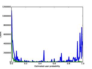
Figure 4: Distribution of ratings of user-relatedness on our corpus (blue) and for our stop list (green), the latter multiplied by 5).

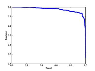
Figure 5: Precision versus recall for our training set.

The processing time on our corpus was around 10,000 hours (a total across multiple processors) to run Bulk Extractor on 63.6 terabytes of image data, and 4 hours for the subsequent address analysis.

5. Visualizing email networks

Once we have excluded uninteresting email addresses, we can see more clearly the connections between users. Even though most users of drives in our corpus employed mail servers, we saw many email addresses on our drives.

5.1. Measuring the dissimilarity between addresses

A key idea that will help visualize connections between email addresses is the notion of their dissimilarity. Using this, we can approximate a metric space of all addresses where dissimilarities are shown as distances, and then seek clusters in it.

Several ways to measure dissimilarity were explored in this work:

· Absolute value of the difference in offsets in the storage in which the addresses were found (McCarrin, Green, and Gera, 2016), or . The difference in offsets would seem to be a good measure of dissimilarity since addresses found nearby are likely to be within the same line of the same file and thus related.

· Dissimilarity of the words in the two addresses when they are split using the methods of section 4.4. Address pairs with shared domain/subdomain lists are weakly associated. Address pairs with shared username words are more strongly associated since they suggest aliases and human relatives. Aliases are increasingly common online as people manage multiple mail services (Gross and Churchill, 2007). We estimated word dissimilarity by a weighted sum of the Jaccard metric values on the username and domains separately, as where means the words of the username part of address i, means the domains and subdomains of address i, and J is 1 minus the number of words in the intersection of the two word lists divided by the number of words in the union of the two word lists. We excluded country codes and the final subdomain from the domain word lists since they are broad in their referents, and we excluded integers and one and two-character words from the username wordlists. For example, between "john.smith@groups.yahoo.com" and "jrsmith@mail.yahoo.com" we computed a dissimilarity of . The weights 60 and 20 were picked to be consistent with the offset differences, and say that similarities in usernames are three times more important than similarities in domains.

· Dissimilarity based on lack of co-occurrences over a set of drives. We used where is the number of drives with the pair of addresses i and j. Again, this was fitted to be consistent with the degrees of association in the offset differences. The rationale is that pairs that occur together more than once on drives have some common cause. Note this formula needs to be adjusted for differences in the size of corpori.

· Whether two addresses were not within the same file, as a better way of scoping a relationship than using offset difference alone. We used the Fiwalk tool as mentioned in section 4.2. As noted, few addresses were within files, which limits the applicability of this measure. Nonetheless, there were correlations for certain kinds of files but not others. This will be a subject of future work.

· Whether two addresses were not in the same message. This idea has been used to distinguish legitimate addresses from spam addresses (Chirita, Diederich, and Nejdl, 2005).

The first three methods are useful for our corpus. The fourth and fifth require additional information not always easy to get. Note that only the first two of these dissimilarity measures are metrics (distances) because the last three can violate the triangle inequality . Nonetheless, we can still get useful visualizations from the last three.

5.2. Testing the dissimilarity measures

An important question is how well these dissimilarity measures represent the association of two addresses. This is a challenging question for our corpus because we do not know the people that used nearly all the addresses. Nonetheless, one simple indicator is the correlation of the dissimilarity measures with the ratings of user-relatedness obtained by the methods of part 4, since similar ratings suggest association. Figure 6 plots the absolute value of the difference in our ratings against the absolute value of the difference in offsets for our full corpus; Figure 7 plots the same against our measure for word dissimilarity; and Figure 8 plots the same against our measure of co-occurrence dissimilarity. Though the data is noisy, there are correlations up to 25 on offset deviation, up to 50 on word distance, and up to 25 (representing 7 co-occurrences) on co-occurrence dissimilarity. So it appears that these three measures are useful measures of association at low values and can be plausibly treated as distances.

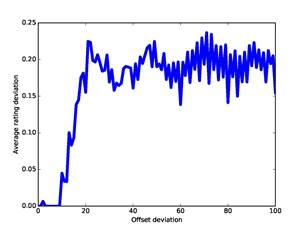
Figure 6: Ratings deviation versus offset deviation for the full corpus.

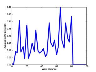
Figure 7: Ratings deviation versus word distance for the full corpus.

Based on these results, we formulated a combined dissimilarity measure for addresses on the same drive. We did not include the co-occurrence dissimilarity because we saw few instances of co-occurrence in our corpus once we eliminated nonuser addresses. But we could use the offset difference and word dissimilarity. They should be combined so a low value on one overrides a high value on the other since a low value usually has a

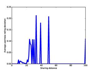
Figure 8: Ratings deviation versus sharing dissimilarity (distance) for the full corpus.

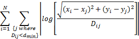
reason. That suggests a "consensus dissimilarity" between address i and address j:

where is offset dissimilarity and is the word dissimilarity, provided either or . Figure 9 shows the distribution of the combined dissimilarities we found between all pairs of email addresses in our corpus. To limit computation, we only computed word similarity for addresses within an offset of 1000. Note the curve is concave upwards, which suggests a relatively even spacing of points in a metric hyperspace. Before calculating this it was important to eliminate duplicate successive addresses in the Bulk Extractor output to prevent their overweighting, since there are many of these due to automated software contacts: The most common such address, CPS-requests@verisign.com, occurred 1.2 million times total in successive entries due to the frequency of certificate stores.

5.3. Experiments with familiar data

To get a better understanding of the effectiveness of our methods, we took drive images of 11 drives of people at our school where the drive owners agreed to explain their connections. We used dissimilarities computed using the methods of the last section and then placed addresses in a two-dimensional space in a way most consistent with the dissimilarities. Two-dimensional space was used for ease of visualization. Many algorithms

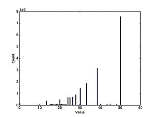
Figure 9: Histogram of all calculated dissimilarities for pairs of addresses in our corpus.

can fit coordinates to distances, and visualization does not need an optimal solution. We thus used an attraction-repulsion method to find x and y values that minimize:

for the consensus dissimilarity values described the last section, and with . We used a log ratio error rather than the least-squares dissimilarity error so as to not unfairly weight points with a big dissimilarity from others (a weakness of much software for this problem). There are an infinite number of equally optimal solutions to this minimization differing in translation and rotation.

We show here data from a drive of one of the authors that had been used from 2007 to 2014 for routine academic activities and also had files copied from previous machines going back to 1998. It was a Windows 7 machine and had 1.22 million email addresses on it of which only 52,328 were unique. Many addresses were not user-related (76 of the 100 most common, for instance), so it was important to exclude them to see explicit user activity.

Figure 10 and Figure 11 show the results of position optimization for a subset of addresses on this drive, those of the first author or addresses connected to the first author by a less than 50.

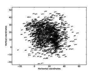
Figure 10: Visualization on a sample drive of addresses of first author and directly-connected other addresses.

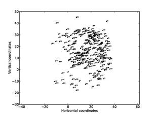
Figure 11: Visualization on a sample drive of addresses of first author and directly-connected other addresses, after filtering to eliminate nonuser addresses.

Usernames have been replaced with numbers to preserve privacy. Figure 10 shows the graph found on the complete subset of addresses (1646 in total), and Figure 11 shows the graph after elimination of the nonuser addresses from the subset (313 in total). Nonuser elimination did help clarify the data, and enables us to better distinguish the author's aliases and close associates centered at (10,10) from other members of the author's department to the right and above, and from other contacts that are outliers below and above. The tendency to form circular arcs is due to the limited amount of distance data below the threshold for users other than the author. This processing took around 70 hours on our full corpus.

6. Visualizing similarities between driveS Using Addresses

Besides graphing connections between individual email addresses, it is useful to graph connections between drives based on the count of their shared email addresses. Now the nodes will be drives and the counts provide a measure of drive-owner association since users that share many addresses are likely to be similar. This should provide more reliability in associating drive owners since the comparison can draw on thousands or millions of data points. It can also provide an alternate way to see hidden social networks not apparent from explicit links. We can do this for the full set of addresses on drives to see shared software, or we can eliminate nonuser addresses first using the methods of section 4 to see just the personal contacts.

6.1. Fitting drive distances

One simple approach to measuring drive similarity based on shared email addresses is to let be the number of addresses on each drive, and be the number of addresses they have in common. Treat the set of addresses on the drives as an independent random sample from some large population of N. Then for drives i and j, counts and , and intersection count , the independence assumption implies that , allowing us to estimate a virtual . A simple additional assumption we can use to estimate dissimilarity is that points of the population of addresses are evenly spaced in some region of hyperspace. Here we want to visualize the dissimilarities in two dimensions, so assume the points of the population are evenly spaced within a circle or square. Then if we increase the area of the circle or square by a factor of K, the radius of the circle or the side of the square increases by a factor of , and the dissimilarities between random points in the circle or square increase by the same factor. Hence the dissimilarity between two drives can be estimated as . This does not become zero when the two sets are identical, but overlaps between drive addresses were quite small in our corpus so this case was never approached. This becomes infinite when , and is unreliable when is small, so distances need to be left undefined in those cases. Then we can use the same optimization formula in section 5.3 for finding coordinates from distances. Figure 12 shows results for drive similarity using the filtered (user-related) addresses where ; we used the K-Means algorithm with K=13 to assign drives to clusters, and then colored the clusters. The differences between clusters were subtle from inspection of their addresses, so we appear to have discovered some new groupings in the data. This processing only took a few minutes once we had the shared-address data referenced in section 5.

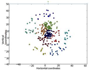
Figure 12: Drive clustering (colors) using count of shared addresses, for distance .

6.2. A social-network approach

An alternative visualization technique is to calculate a containment score (Broder, 1997) based on the size of the intersection of sets of features divided by the number of features of the smaller set, or where n is the count of features on a drive. We can then create a topological view of the connections between drives in which drives are represented as nodes and the weight of the edges between nodes denotes the value of the containment score between the drives to which they correspond. Figure 13 shows an example of this method for the email address-based connections on an example drive.

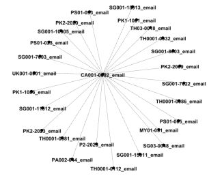
Figure 13: The degree distribution for emails on a drive.

To display and manipulate the resulting graphs we used the open-source graph analysis and visualization tool Gephi (http://gephi.org). Visualization makes it easier to identify clusters of related items; the tool also provides a variety of filtering strategies and layout algorithms.

To reduce noise, we focused on the core of the networks (Borgatti and Everett, 2000). Generally, the k-core is defined as a subgraph whose nodes have at least connections to each other and fewer than to any of the other nodes in the network. The core is the non-empty k-core with the maximum value of k. It often identifies the key players in a social network. Further filtering by degree centrality highlights the most connected nodes within the core.

6.3. Results of the social-network approach

To establish a baseline picture of relationships between drives, we calculated shared-address counts between drives using addresses as features and eliminating the addresses below the 0.3916 probability. Table 7 shows the distribution of sharing counts between drive pairs. The frequencies do not follow a Zipf's Law 1/k trend at higher counts but reflect meaningful associations.

The graph of drive similarity based on common email addresses has 3248 nodes and 447,292 edges. Its degree distribution follows the expected power law that we see in big data (see Figure 14). It shows that while there are some drives with high

Table 7: Sharing counts of addresses between drives and their frequencies of occurrence.

Shared count	Frequency	Shared count	Frequency
1	401201	2	27888
3	8089	4	4169
5	2130	6	1288
7	1270	8	1563
9	1955	10-14	2801
15-19	963	20-29	870
30-99	2167	100-999	667
1000-9999	126	10000	45

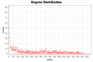
Figure 14: The degree distribution of the drive image similarity network, where connections are shared email addresses.

degree of 850, there are over 90 drives of degree 0, meaning that they have no shared email addresses with any other drives. However, the average degree is 260.96, so there are enough correlations.

Screening the network of drives having at least one address in common, by k-core with k=298, we obtain a hairball of 1214 nodes and 226,180 edges, and at k=299 the whole core vanishes. The 298-core is therefore the core of the graph and identifies the most connected subgraph (with each node having 298 connections or more to the other 1214 nodes in the core). The nodes in this set all have a similar position in the network and a similar relative ranking to the other nodes in the core.

However, further analyzing the 298-core of the network, we identified three key drives that all share email addresses with the leftover 43 drives as shown in Figure 15. Each of these drives has at least 439 connections. Such a complete bipartite graph is an unusual pattern of correlation in real networks, since the three drives do not have a high correlation to each other, but a similar high correlation to the other 43 drives.

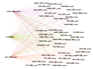
Figure 15: The neighborhood of the highest three degrees in the core (with "communities" or key subgraphs indicated by colors).

Figure 16 shows the neighborhood of the highest 5 degree nodes in the core. We included a few other high degree nodes to see if they showed an interesting pattern, which was indeed observed for the top 9 nodes of the core.

Degree centrality does not necessarily equate to importance, and the more central nodes in a network can be the most redundant as has been observed here. Nonetheless, these topological visualizations can be helpful in seeing a network in a different way, screening data when there is too much, and analyzing the important nodes. This makes a useful supplement to analysis based on individual node properties.

7. Conclusion

Electronic mail addresses alone can provide useful information in a forensic investigation even without the associated mail. Nonetheless, many email addresses are uninteresting for nearly all investigations, and we have shown some simple

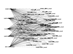
Figure 16: The neighborhood of the highest five degrees in the core.

methods that can exclude them reliably. We have shown this significantly improves the ability to see connections between email addresses on a diverse corpus, and enables us to see new phenomena in the connections between addresses and drives viewed in two different ways. Such information can be combined with other kinds of connection information found on a drive such as telephone numbers, Internet addresses, and personal names to get a good picture of the social context of its user.

Acknowledgements

Janina Green collected the data described in section 5.3. The views expressed are those of the authors and do not represent the U.S. Government.

REFERENCES

[1] Borgatti, S., & Everett, M. (2000). Models of core/periphery structures. Social Networks 21 (4), 375-395.

[2] Broder, A. (June). On the resemblance and containment of documents. Paper presented at the IEEE Conference on Compression and Complexity of Sequences, Positano, Italy, June (pp. 21-29), June 1997.

[3] Bulk Extractor 1.5. (2013). Digital corpora: Bulk Extractor [software]. Retrieved on February 6, 2015 from digitalcorpora.org/ downloads/bulk_extractor.

[4] Chirita, P.-A., Diederich, J., & Nejdl, W. (2005). MailRank: Using ranking for spam detection. Paper presented at the Conference on Information and Knowledge Management, Bremen, Germany, October-November (pp. 373-380).

[5] Garfinkel, S., Farrell, P., Roussev, V., & Dinolt, G. (2009). Bringing science to digital forensics with standardized forensic corpora. Digital Investigation 6 (August), S2-S11.

[6] Gross, B., & Churchill, E. (2007). Addressing constraints: Multiple usernames, task spillage, and notions of identity. Paper presented at the Conference on Human Factors in Computing Systems, San Jose, CA, US, April-May (pp. 2393-2398).

[7] Holzer, R., Malin, B., & Sweeney, L. (2005). Email alias detection using social network analysis. Paper presented at the Third International Workshop on Link Discovery, Chicago, IL US, August (pp. 52-57).

[8] Klensin, J, & Ko, Y. (2012, February). RFC 6530 proposed standard: Overview and framework for internationalized email. Retrieved February 4, 2016 from https://tools.ietf.org/html/rfc6530.

[9] Lee, S., Shishibori, M., & Ando, K. (2007). E-mail clustering based on profile and multi-attribute values. Paper presented at the Sixth International. Conference on Language Processing and Web Information Technology, Luoyang, China, August (pp. 3-8).

[10] McCarrin, M., Green, J., & Gera, R. (2016). Visualizing relationships among email addresses. Forthcoming.

[11] Newman, M. (2004). Fast algorithm for detecting community structure in networks. Physical Review E, 69, (7), p. 066133.

[12] Polakis, I., Kontaxs, G., Antonatos, S., Gessiou, E., Petsas, T., & Markatos, E. (2010). Using social networks to harvest email addresses. Paper presented at the Workshop on Privacy in the Electronic Society, Chicago, IL, US, October (pp. 11-20).

[13] Rowe, N., Schwamm, R., & Garfinkel, S. (2013). Language translation for file paths. Digital Investigation, 10S (August), S78-S86.

[14] Zhou, D., Manavoglu, E., Li, J., Giles, C., & Zha, H. (2006). Probabilistic models for discovering e-communities. Paper presented at the World Wide Web Conference, Edinburgh, UK, May (pp. 173-182).