14th ICCRTS: C2 and Agility
Wireless Sensor Networks for Detection of IED Emplacement
Topic 2: Networks and Networking
Neil C.� Rowe (point of contact), Matthew O'Hara, and Gurminder Singh
Code CS/Rp, 1411 Cunningham Road
Naval Postgraduate School, Monterey , CA 93943 USA
ncrowe@nps.edu, (831) 656-2462
Abstract
We are investigating the use of wireless nonimaging-sensor networks for the difficult problem of detection of suspicious behavior related to IED emplacement.� Hardware for surveillance by nonimaging-sensor networks can cheaper than that for visual surveillance, can require much less computational effort by virtue of simpler algorithms, and can avoid problems of occlusion of view that occur with imaging sensors.� We report on four parts of our investigation.� First, we discuss some lessons we have learned from experiments with visual detection of deliberately-staged suspicious behavior, which suggest that the magnitude of the acceleration vector of a tracked person is a key clue.� Second, we describe experiments we conducted with tracking of moving objects in a simulated sensor network, showing that tracking is not always possible even with excellent sensor performance due to the ill-conditioned nature of the mathematical problems involved.� Third, we report on experiments we did with tracking from acoustic data of explosions during a NATO test.� Fourth, we report on experiments we did with people crossing a live sensor network.� We conclude that nonimaging-sensor networks can detect a variety of suspicious behavior, but implementation needs to address a number of tricky problems.
This paper appeared in the Proceedings of the 14th International Command and Control Research and Technology Symposium, Washington, DC, June 2009.
1. Introduction
Improvised explosive devices (IEDs) are an increasingly serious military threat.� We are investigating to what extent wireless sensor networks can help.� Detection of emplaced IEDs is very difficult as is witnessed recently in Iraq and Afghanistan, where results with remote sensing have been disappointing.� Attacking the network that emplaces IEDs, a current focus of the Joint IED Defeat Organization (JIEDDO), is also very difficult because of the decentralized nature of the insurgent networks employing IEDs, and the network's broad scope risks considerable collateral damage when attacked.� So it appears important that we also attack IEDs during emplacement, during these inherently suspicious actions.� We are exploring to what extent this can be automated to reduce the need for dangerous patrols.
Much that has been written about lessons from IEDs in Iraq and Afghanistan supports this approach (Wilson, 2007).� Technology has been tried for "clearing roads" using focused sensing over a route in advance (Chisolm, 2008), but this misses some IEDs and does not prevent IED emplacement after the road has been cleared.� (Atkinson, 2007) points out the importance of adaptivity in combatting IEDs, since the technology of IEDs is often simple and easy to make variations upon.� This means that useful long-term IED countermeasures must be able to collect a broad range of information over a long period of time, something sensor networks can provide.� (Saletan, 2007) points out the importance of having persistent surveillance over time to combat the simplicity of the IED technology.��
Traditionally, automation of surveillance means using cameras.� But this requires considerable human monitoring, and such monitoring is tedious and highly prone to errors (Hackwood and Potter, 1998).� Attempts to automate it further with automated visual processing suffer from high error rates at understanding a wide range of activities in three dimensions, and problems with occlusion and image resolution.� So we have been exploring wireless nonimaging-sensor networks for detection of emplacement.� Such networks can detect phenomena related to IEDs such as excavation (through acoustic and seismic sensors), presence of ferromagnetic materials (through magnetic sensors), and can do rough tracking of people passing through the sensor field (though acoustic, infrared, and seismic sensors).� Such sensors can be significantly cheaper than cameras, can avoid occlusion, can avoid confusion of depth (Valera and Valestin, 2005), can violate privacy less of those tracked, can be easier to conceal from adversary countermeasures, and can be distributed over large areas to provide uniform coverage.
Sensor networks can be deployed in several ways to aid in combatting the IED threat.� They can be deployed for persistent surveillance of an area (Pendall, 2005), where they alert commanders to potentially suspicious behavior that can then trigger the turning on of cameras to record further information or can trigger manual inspection by police or military personnel.� They can be used for a small area such as a checkpoint or for broad-scale surveillance of a larger area such as a neighborhood.� They can be managed by a small unit for defense of their perimeter, or they can be managed by a larger organization as part of comprehensive intelligence gathering.� Since management entails analysis of data and some judgment, specialized personnel must assist in monitoring a deployment.
The work reported here investigates some key issues with sensor networks for the IED problem.� We conclude that accuracy can be obtained, but it requires care in the design and setup of the sensor network.� This work builds on our previous experiments with wireless sensor networks (Rowe, 2005; Sundram, Poh, Rowe, and Singh, 2008) using a testbed of Crossbow sensors in a public area at our school.
2. Clues for suspicious behavior in video
We first must choose clues to look for.� Seismic clues to excavation can be quite obvious: Look for repeated actions with a one to ten second period.� However, IEDs can also be emplaced quickly without excavation by being dropped onto roads.� Usually when that occurs there were some unusual actions that would have been obvious to an observer.� So the question is what reasonably specific clues we could pick up with a sensor network.� Because of our focus on sensor networks, we will not look for background changes as clues to suspicious behavior (Gibbins, Newsam, and Brooks, 1996), something more appropriate for visual surveillance.� We also want sensor networks to cover large areas rather than provide close-up surveillance of targeted areas, so we will not try to recognize human gestures (Merservy et al, 2005).
Our focus also will be on suspicious behavior, not anomalous behavior, so we will focus on clues that relate to deception.� Good work has been done on detecting anomalous visual behavior (Lee, Yu, and Xu, 2003; Jan, 2004; Barbara et al, 2008; Wiliem et al, 2008) by analyzing characteristics of a human motion trajectory using a variety of features.� However, there are many reasons why human motion can be anomalous that have nothing to do with insurgency or terrorism.� Systems focused on anomaly detection may be helpful for policing but are likely to generate too many false alarms to be helpful for IED detection.� Instead, we need to focus on clues to deliberate deception such as concealment and abrupt changes in goals.�
To study this problem, we obtained a video dataset from the Force Protection Surveillance System Project at the U.S. Army Research Laboratory.� It had training sequences of around 50,000 frames and a set of� 53 test sequences of a total of 71,236 frames.� They showed both normal and staged activities in a parking lot.� The staged activities included loitering, carrying of objects, emplacing and removing of objects, people in unusual places, and vehicle stops in unusual places.� Video was obtained as pairs from two fixed-position side-by-side cameras, one color and one infrared; our analysis was generally more accurate with the easier segmentation of the infrared video.� We had ground truth as to deliberately staged suspicious actions in the video, in the form of text annotations for each image sequence.� We used standard video-processing methods to track the people and vehicles that were moving in the images.� We constructed a synthetic background image for each image sequence representing the median color at each pixel in the sequence.� We then subtracted each image from the background and segmented using a threshold that yielded 95% of the pixels of moving objects that we could see ourselves.� Relaxation methods were used to find the best matches between objects in successive frames of the video.
We automated and tested seven factors that relate to suspiciousness.
- infrequency of visit to that location
- atypicality of speed over all observed speeds (adjusting for distance from the camera)
- atypicality of the velocity vector at that location
- the norm of the acceleration vector a(d) where d is the
time window, over 0.2, 0.4, 0.8, 1.6, and 3.2 second time intervals,
defined as
 .� �����������We chose d
to correspond to 0.2, 0.4, 0.8, 1.6, and 3.2 time windows; since images
were taken approximately 0.2 seconds apart, this corresponded to d=1, d=2,
d=4, d=8, and d=16.� Examination of different time scales in important
because some suspicious activities like theft take place quickly (Powell,
Tyska, and Fennelly, 2003) but others like loitering occur over an
extended time period.
.� �����������We chose d
to correspond to 0.2, 0.4, 0.8, 1.6, and 3.2 time windows; since images
were taken approximately 0.2 seconds apart, this corresponded to d=1, d=2,
d=4, d=8, and d=16.� Examination of different time scales in important
because some suspicious activities like theft take place quickly (Powell,
Tyska, and Fennelly, 2003) but others like loitering occur over an
extended time period. - fraction of apparent concealment (1 minus the ratio of size to the maximum size of the region along its path), since criminals want to hide (Wood, 2000)
- shortness of the path
- "contagion" by other nearby suspicious paths since nearness suggests social interaction.� Identifying anomalous social interactions helps too (Panangadan, Mataric, and Sukhatme, 2004) but there were few social interactions in our data.
The first four factors were adjusted by estimated distance
from the camera, based on fitting to the observed width of people in training
sequences.� The weights on the seven factors in our experiments were set after experiments
to 0.04, 0.24, 0.08, 0.24, 0.16, 0.04, and 0.20, respectively.� To make
weighting easier, following standard practice with artificial neural networks,
a sigmoid function ![]() �mapped metrics to
probabilities before taking the weighted average where μ is the scale.� Parameters
μ were obtained by experiments with the control dataset.� The weighted sum
of the factors is the estimated suspiciousness for each path segment, and can
be averaged over a path to estimate the path suspiciousness.� Figure 1 shows an
example track for an infrared sequence where a subject wanders by a trash can
(bottom left), throws something in, wanders around a vehicle (upper right), and
then leaves; redness indicate estimated suspiciousness.
�mapped metrics to
probabilities before taking the weighted average where μ is the scale.� Parameters
μ were obtained by experiments with the control dataset.� The weighted sum
of the factors is the estimated suspiciousness for each path segment, and can
be averaged over a path to estimate the path suspiciousness.� Figure 1 shows an
example track for an infrared sequence where a subject wanders by a trash can
(bottom left), throws something in, wanders around a vehicle (upper right), and
then leaves; redness indicate estimated suspiciousness.
Performance on the test set was measured by precision (fraction of correctly identified suspicious behavior in all the behavior identified as suspicious) and recall (fraction of correctly identified suspicious behavior of all the suspicious behavior visible).� The threshold (0.3 for most experiments, and 0.7 for experiments with just the acceleration factor) was chosen to keep precision and recall values close for a more accurate estimation of the F-score (the harmonic mean of recall and precision, a standard metric for classification tasks).� Assessment was done by manual inspection of summary pictures for each sequence, and using the ground-truth descriptions.� 161,023 nontrivial path segments were identified in the images.
Figure 1: Example suspiciousness analysis for an infrared image sequence.
We obtained an F-score of 0.64 on color sequences and 0.66 on infrared sequences using all factors, and 0.59 and 0.60 respectively with just the acceleration factor.� This means we could get roughly 40% false alarms with 40% false negatives.� This supports our hypothesis that gross body motion, and the acceleration factor in particular, is sufficient to indicate most suspicious activities.� This supports the value of wireless sensor networks for detection of suspicious behavior because they reduced by a factor to 40% the amount of required visual inspection for suspicious behavior in the experimental task.
3. Simulation of tracking by a sensor network
To explore the capabilities and limitations of sensor networks for tracking of objects, we built a simulator in the Matlab language.� This enabled us to see how much of tracking error could be due to the algorithms themselves.� Since our subsequent work (see section 5) used Crossbow sensors with magnetic, passive-infrared, and acoustic modalities, we simulated those signals.
Our simulation experiments used a rectangular grid of sensors for simplicity.� While the Crossbow sensors have some directional characteristics, these anisotropic effects are inconsistent and hard to model.� So our simulator assumed isotropic detection using only signal strength and time of arrival.� We assume a calibration phase can adjust for inherent differences in the detection strength and clock times at each sensor. by using a signal source of a fixed known strength sent across the network, similarly to the experiments described in section 5.
We explored using both the signal strength and time of arrival to do tracking.� (Phase shift can also be used for some signals.)� The mathematics of each are quite different.� This means they tend to be independent, and using both provides better accuracy than using one alone.
3.1. Tracking by signal strength
Signal strength was assumed to be additive from all sources.� Following discussions of acoustic, seismic, and magnetic signals in the literature, each signal strength was assumed to be a random factor plus i/(m+d)^2, where i is the intensity of the source, d the distance from the source to the sensor, and m the minimum radius from the source which is a feature of each sensor.� Such an inverse-square law is a good model for many sensing modalities since, with many wave and field phenomena, signal strength is proportional to the area of a sphere centered at the source and touching the sensor.� We assume the sensor field is placed in a small and mostly unobstructed area like a public square, so that reference signals are not necessary as in (Zarimpas et al, 2005).� Determination of a minimum distance is necessary to avoid unstable behavior with very-near sources.
Our simulator creates random object tracks in the sensor space and then calculates the associated signal strengths at evenly spaced time points to provide test cases for analysis.� Analysis then tries to reverse the process and infer the source locations from the strength patterns.� Work addressing a similar problem of triangulation on signal strengths with different techniques is (Figueiras, Schwefel, and Kovacs, 2005).� Figure 2 shows an example display of the simulator where green circles represent the sensors (and their size indicates their received signal strength), blue (larger) circles represent the objects being tracked, and small purple circles represent their inferred positions using just signal strengths as explained below.� The closer the purple circles to the blue circles, the better the tracking; in a few cases of excellent tracking, the purple is within the blue.
Figure 2: Example snapshot of the tracking simulator with eight tracked objects.
Our first approach to localization used a classic steepest-descent optimization technique.� Unfortunately, it is difficult to ensure that the optimization will converge since the parameter space has many local minima.� Convergence is particularly a problem if the initial estimates of the tracked objects are not close to their actual locations.� In experiments with an average of two random constant-speed tracks across a 3 by 3 sensor array in the form of a square grid, convergence failed 86 out of 110 times when assigning sources initially to the local maxima of the signal in the sensor grid.
We got better performance by using equations based on the observed ratio of signal strengths, a variation on the approach of (Lee et al, 2006).� If we assume for an initial approximation that the observed signal strength is due only to each sensor�s nearest source (effects fall off fast with an inverse square), then for two sensors 1 and 2 nearest the same signal:
![]()
Here s represents signal strength,
m represents the minimum-distance factor, (x,y) is the position of the tracked
object, and![]() and
and![]() are the
coordinates of the sensors.� Rearranging this gives an equation of a circle for
the locus of points on which the sensor could lie.� The center and radius of
this circle are:
are the
coordinates of the sensors.� Rearranging this gives an equation of a circle for
the locus of points on which the sensor could lie.� The center and radius of
this circle are:

We can intersect two circles (from three sensors) to reduce the locus of two points.� With more than three sensors, we can find the "consensus center" by finding the set of all intersection points and repeatedly removing the furthest point from the centroid of the set until we have two points of which to take the centroid.� Once we have inferred the source points, we can compute their signal strengths, then recompute the positions and strengths iteratively until accuracy is sufficiently good.� We can also subtract out effects of the further-away sources at each sensor once we have reasonable estimates of all the source positions.
For this method of estimation of track locations to work, we
must be careful to choose readings of signal strength from at least four sensor
nodes including the local maximum, which gives us three circles to intersect.� It
is also important to obtain at least three different horizontal and three
different vertical values in the sensor readings, and signals strengths that
are not identical or near-identical, to avoid an "ill-conditioning"
problem in which solution accuracy is poor because the denominator![]() is near zero.� We thus chose the two horizontal and two vertical neighbors for
each sensor in the square sensor grid, except along borders of the grid where we
used points deeper within the grid to obtain three along each dimension.� This
gives five sensor readings and six circles to intersect.
is near zero.� We thus chose the two horizontal and two vertical neighbors for
each sensor in the square sensor grid, except along borders of the grid where we
used points deeper within the grid to obtain three along each dimension.� This
gives five sensor readings and six circles to intersect.
Note that this approach is well suited to local computation on the sensor grid since we only need to bring together data from five neighboring sensors.� Eventually, however, the tracking results must be collected by a central node.� This approach does not necessarily require a uniform grid.
We ran our simulation to obtain upper bounds on performance of a real sensor network.� Table 1 shows results for a 100 by 100 grid over a time interval of 20 seconds, averaged over 100 runs for each entry.� A square boundary around the sensor area was constructed whose distance from the nearest sensors was the same as the distance between neighbor sensors; random starting and ending locations were chosen on the boundary.� Random starting times were chosen in the 20-second interval, but tracks could continue after 20 seconds as necessary to reach their goal points, and the results covered this extra time.� The average velocity per unit of the track was 10 and the average strength was 5 in all these experiments.� The first six columns of Table 1 give the independent (experimental) variables, and the last four columns give results.� "V sd" is the standard deviation of that velocity for the track (for variation perceived by all sensors), "s sd" the standard deviation of that strength (for variation perceived by all sensors), "si sd" is the standard deviation of the observed strength at each sensor for a signal of fixed strength, and "h dev" the average random deviation in radians of the track heading from the ideal heading towards its goal point (to model wandering).� "Tracks" means how many different tracks were created during the time interval.� The two numbers for each entry represent the average distance error in the track position and average error in the logarithm of the strength of the track at that position; smaller numbers for these are better.
It can be seen that our circular optimization definitely improves the estimate of track positions, even with eight tracks in the sensor area simultaneously when it can more easily get confused.� Doing it more than once does not help (despite its need to guess locations of far tracks).� Doing a subsequent optimization using the gradient formulas shown above actually worsens performance considerably on the average, illustrating how ill-conditioned the problem is.� Varying the average velocity and signal strength of the tracks and their variance had little effect on performance.� However, increasing the error with which individual sensors perceived the same signal did naturally degrade performance; just a 40% error in perceived signal strength made circle optimization significantly less effective for improving track-location estimates, though not so much on improving signal-strength estimates.� Performance was not degraded as much as the introduced error, suggesting that the sensor consensus helps reduce errors.
Table 1: Simulation results for straight tracks across a square sensor grid.
|
|
grid |
v sd |
s sd |
si sd |
h dev |
1 track |
2 tracks |
4 tracks |
8 tracks |
|
Track locations are signal peaks |
10x10 |
0 |
0 |
0 |
0 |
1.826, 0.324 |
3.189, 0.541 |
5.738, 0.955 |
10.935, 1.544 |
|
Track locations from circle estimation |
10x10 |
0 |
0 |
0 |
0 |
0.000, 0.000 |
0.369, 0.026 |
1.378, 0.108 |
6.042, 0.447 |
|
Same |
10x10 |
5 |
2.5 |
0 |
0.3 |
0.000, 0.000 |
0.278, 0.021 |
1.217, 0.102 |
5.186, 0.437 |
|
Same, estimation done twice |
10x10 |
5 |
2.5 |
0 |
0.3 |
0.000, 0.000 |
0.278, 0.024 |
1.217, 0.114 |
5.186, 0.459 |
|
Same, estimation then traditional optimization |
10x10 |
5 |
2.5 |
0 |
0.3 |
0.000, 0.000 |
1.926, 0.020 |
9.093, 0.189 |
24.698, 0.959 |
|
Same, circle estimation |
4x4 |
5 |
2.5 |
0 |
0.3 |
0.000, 0.000 |
1.841, 0.063 |
9.275, 0.309 |
28.292, 1.094 |
|
Track locations are signal peaks |
10x10 |
5 |
2.5 |
2 |
0.3 |
1.851, 0.324 |
3.042, 0.521 |
5.411, 0.869 |
10.551, 1.472 |
|
Same, circle estimation |
10x10 |
5 |
2.5 |
2 |
0.3 |
0.805, 0.059 |
1.563, 0.108 |
3.109, 0.216 |
7.405, 0.538 |
These tracking methods did not smooth the inferred tracks by assumed velocity consistency over time, a technique important in applications like radar tracking of aircraft.� Such methods could significantly improve our tracking performance.� However, section 2 emphasized the importance of determination of accelerations.� Seeking more velocity consistency in tracking would hurt estimates of acceleration.
3.2. Tracking by time of arrival
Tracking moving sources by time of arrival of signals at a set of sensors is a familiar technique since it is used by the Global Positioning System.� We can do it by solving a different optimization problem (Kaplan et al, 2006).� However, applying it to sensor networks must depart in a few important ways from the GPS analysis.� We can get times accurate within milliseconds with relatively simple methods, and the times in the experiments reported in section 4 were accurate within 0.025 milliseconds.� This permits, in principle, localization within inches.
The differences in times at which a signal is received are proportional to the differences in distances from the source of the sound.� Thus in a two-dimensional plane, the locus of points of a source based on readings from two sources is a hyperbola.� Three readings from sources reduce the locus to (generally) two points, and four readings reduce it to one point.� However, it is best to obtain as many readings as we can to compensate for inaccuracies, and then use a fitting method like least-squares to minimize to overall error.
Again suppose we have a set of N sensors at locations ![]() �for
i=1 to N.� Assume that corresponding peaks arrive at each sensor at time
�for
i=1 to N.� Assume that corresponding peaks arrive at each sensor at time ![]() .�
We want to minimize:
.�
We want to minimize:
 ��
��
Here c is the average speed of the signal and (x,y) is the position of the tracked object as before.� The derivatives of G are (where "sgn" is the sign of its argument):

The two ratios are equivalent to the cosine (for x) and sine (for y) of the bearing angles from the estimated source location to the sensor.� Thus we can optimize the location of the tracked object by moving its position by a weighted sum of the vectors to each of the sensors.
4. Experiments with acoustic data of explosions
To test our tracking algorithms on real data, we obtained acoustic-sensor records from NATO experiments conducted by the Army Research Laboratory in June 2008 in Bourges, France.� Some sensors were within around fifty feet of one another, and other sensors were at longer distances up to a mile.� Acoustic events were produced by small-arms fire, mortars, and other kinds of explosions.� Since many of the sensors were close to the trajectory of the propelled projectile, much of the acoustic data shows separately a shockwave and a subsequent muzzle blast.� Loud noises do occur during IED emplacement.
We analyzed the acoustic signals to extract key features that we hoped would aid in matching between data from different sensors.� Our primary focus was on the simplest features of the signal.� The raw data was sampled at 40,000 hertz.� We subtracted the signal from its mean over the entire interval, calculated the sum of the absolute values of the signal over every tenth of the second, and found the mean of these values.� We then found all tenth-second intervals whose sum exceeded this mean, except when preceded by another such interval, and identified them as the "peaks".� This approach was highly accurate at identifying peaks.� For each we computed its time, height, largest frequency of the Fourier spectrum in the 0.5-50 hertz range, log of the Fourier magnitude at that peak, and mean log of the Fourier magnitude over its spectrum.� We chose these features because they are important in distinguishing the key dimensions of low-frequency impulses like explosions.� If we obtained more than five peaks from a sensor-event pair, we used only the five largest.
Figure 3 shows an example of the localizations possible using signal strength alone from all sets of four sensors drawn from twenty and a particular explosion.� It can be seen that while there are circular artifacts due to the use of circles in the signal-strength localization algorithm, there is consensus about the source of the explosion being in the lower right.�
Figure 3: Example localization distribution for one explosion in the NATO acoustic data.
We also explored wavelet decomposition of the signal with Daubechies wavelets because of their similarity in shape to the acoustics of explosions.� Fifth-order wavelet decomposition appeared to be the best in previous work on similar sounds of explosions (Hohil, Desai, and Morcos, 2006) in reducing background noise, and worked well for our own previous work in distinguishing types of artillery by their sounds.� The features we used were based on energy ratios around the peak, a standard technique for identifying weak signals in noisy data.� We used these factors (normalized to have a mean of zero and a standard deviation of 1):
- Log of ratio of energy before and after peak for Level 5 approximation
- Log of ratio of energy before and after peak for Level 5 details
- Log of ratio of energy before and after peak for Level 4 details
- Log of ratio of energy before and after peak for Level 3 details
- Frequency with maximum norm in the Fourier minimum
Unfortunately, results using wavelet decomposition were disappointing: Matching accuracy between signals did not significantly increase when we used parameters from these decompositions instead of the previously described features.� So we did not pursue this approach further.
We used both the signal strength and the time to localize the acoustic sources using the algorithms described in the last section.� Neither performed very well on this data, though the signal-strength approach worked better.� This is disappointing because the time data was quite accurate because it was obtained with a 40,000-hertz sampling rate.� We can only conclude that the matching of peaks was too error-prone to be useful.� Although this technique worked fine on our previous project, it appears that the NATO signals were too noisy, and too subject to echoes and reverberations, to be successful with our approach.� Note however that echoes and reverberations are more a problem with acoustic phenomena having shockwaves, and should be less a problem with the mostly quiet sounds of stealthy IED emplacement.� Also note that putting acoustic sensors closer together, say within ten meters, should eliminate most of the matching difficulties.
5. Experiments with a live magnetic-sensor network
5.1. Introduction
We also conducted experiments with sensor "motes" (devices) from Crossbow; more details are in (O'Hara, 2008).� Useful wireless sensor networks for the IED emplacement problem are "ad hoc" networks (Zhao and Guibas, 2002).� Nodes relay information using a predetermined routing protocol such as ZigBee, which follows the IEEE 802.15.4 standard focusing on low data rates and low power requirements.� Due to the wireless constraint, each network node needs a self-contained power source such as batteries, but these make each mote power-limited and unable to sustain continuous long-term operations.� A "base station" collects data from the nodes and processes it or passes it to a central processor.� The base station has higher power requirements to support both reception and transmission.
Companies such as Crossbow, Ember, and Texas Instruments produce wireless sensor network components and solutions.� Our experiments used the Crossbow MSP410 wireless security system.� The MSP410 package employs sensors used in various wireless intrusion-detection systems, and deploys as part of a robust mesh network of multi-purpose mote protection modules.� The MSP410 system consists of battery-powered motes housing a 433 MHz processor with magnetic, passive-infrared, and acoustic detection capability.� The system also uses a base station module that interfaces to a personal computer.�
The mesh-networking feature of the motes allows motes to communicate with each other.� Additional motes can be added to the network or motes can be removed from the network easily.� Magnetic detection within the motes uses a two-axis magnetic field sensor to detect electronic voltage perturbations around the sensor.� Passive-infrared sensors detect dynamic changes in the thermal radiation environment within immediate vicinity of the sensor.� Motes also contain microphones to detect acoustic changes within its environment.� Each mote contains four magnetic and passive-infrared sensors within a cube housing, to provide nearly 360-degree coverage.�
We focused on detecting magnetic signature since ferrous materials are used in many IEDs and recent progress has made magnetic detection technology cheaper (Bourzac, 2007).� �Experiments used the MSP410 motes, orange safety cones to elevate the motes from the ground, and steel buckets and staples to simulate metallic IED material.� We did three kinds of experiments: configuration, initial-setup, and optimal-configuration.�
5.2. Configuration experiments
The configuration experiments tested the physical attributes, capabilities, and limitations of the Crossbow MSP410 motes.� Configuration experiment 1 kept the metal bucket in a fixed position and the mote was walked along a straight-line path over the bucket.� It was determined that the spacing was too great and the motes had trouble detecting magnetic material unless extremely
close to the mote.� Configuration experiment 2 tested for the angle of sensitivity of the mote, and confirmed that the mote had an 89-degree cone angle, giving it just under full 360-degree coverage.�
Configuration experiment 3 placed the mote 1.5 feet away from a wall.� Metal was placed at varying heights on the wall to determine how high the metal could be detected by the sensor mote.� Results showed that a 2.5 foot height was the maximum height that could be detected.� Configuration experiment 4 placed two motes at varying distances to determine the maximum spacing between the motes that still allowed for detection of magnetic material passing between them.� Results showed that a six-foot spacing was sufficient, and an eight-foot spacing was almost as good.� This means that metal detection is possible when material is within four feet from the mote.�
Configuration experiments 5 and 6 (Figure 4) tested whether the distance from the mote affected the strength of the magnetic readings.� The motes did produce stronger magnetic readings at closer distances.� However, the readings quickly saturated inside of 1.5 feet, which made distance estimation impossible at close distances.
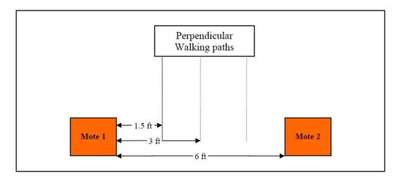
Figure 4: Configuration for experiments 5 and 6.
Configuration experiment 7 showed that large amounts of metal at a specified distance would give the same magnetic reading as smaller amounts of metal at a closer distance.� A keychain placed 6 inches from the mote gave just as strong readings as a bucket placed 3 feet away from the mote, so the inverse square signal strength law did not hold here.� Figure 5 plots observed signal strength versus the amount of ferrous material in some experiments.� It can be seen that the relationship is not linear.� Apparently the configuration of the ferrous materials in different quantities made the readings inconsistent.
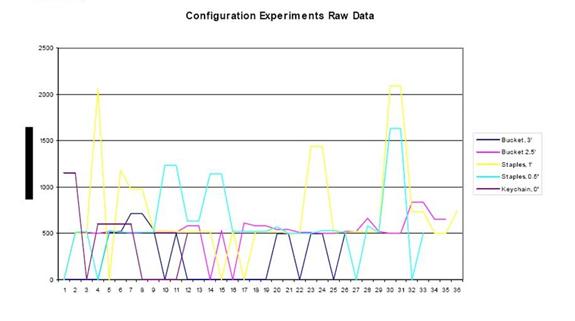
Figure 5: Magnetic signal strength measurements.
5.3. Initial-setup experiments
The initial-setup experiments tested various configurations of a six-mote wireless sensor network to find the best one.� The first experiment (Figure 6) used a rectangular configuration of motes placed at five-meter intervals as shown.� During this experiment, the steel bucket was moved through various paths around the motes, through several repeated tests.� These paths often produced dead spots in which the ferrous material could not be detected.� We concluded that the motes were spaced too far apart.
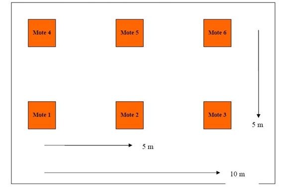
Figure 6: First initial-setup experiment.
Initial-setup experiment 2 tested a hexagonal configuration of motes with mote spacing at five-meter intervals again.� The mote spacing was too great again.� Although magnetic readings were strong near the motes, the strength of readings quickly decreased with increased distance from the motes.� Various walking paths through the network were tested with similar results.�
5.4. Optimal-configuration experiments
�
We obtained better results with the six-node layout shown in Figure 7.� Motes one and five represent an entrance or doorway to an urban building.� The first experiments used a two-foot spacing as shown, and this was later increased to four feet, eight feet, and twelve feet.� Initial experiments used one subject carrying a metal bucket to traverse the network.� The motes could detect magnetic signals from the bucket, and saturation of the signal was when the buckets came close to the motes.�
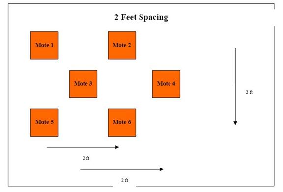
Figure 7: Setup for optimal-configuration experiments.
Later experiments expanded the mote intervals to eight and twelve feet.� Figure 8 shows an example signal strength as a function of time.� While the eight-foot configuration provided reliable and consistent results, the twelve-foot configuration did not.� However, this assumes that motes one and five provide the only entrance point into the network.�
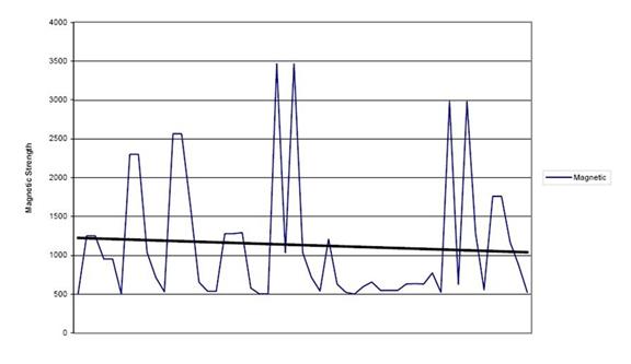
Figure 8: Control subject path in a multi-person experiment: signal strength versus time.
Subsequent experiments increased the number of subjects traversing the network to two or three and varied the amount of metal.� In one experiment, a subject with a small amount of metal walked directly over motes one and two and another subject carrying a metal bucket walked a straight-line path between motes three, four, five, and six, and both subjects generated good readings.�
In another experiment, a subject carried a steel bucket along a predetermined path, while other subjects carried nominal amounts of metal to represent normal conditions like carrying key chains and jewelry.� Some experiments had the subjects walking in parallel.� Other experiments had the subjects traversing the networks in opposite directions.� Final experiments had subjects walking randomly through the network (Figure 9), again measuring signal strength as a function of time.� The experiments consistently detected the steel bucket, and detected small amounts of other kinds of metal were detected when nearby.� Experiments in varying the walking pace showed it did not seem to matter.
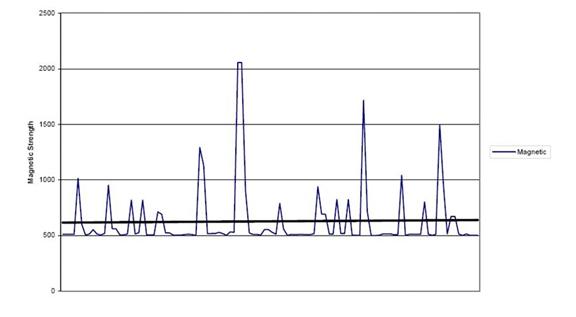
Figure 9: Random subject paths in multiperson experiment: signal strength versus time.
5.5. Conclusions from experiments with the magnetic-sensor network
A wireless sensor network using only magnetic detection is insufficient for the IED problem.� But it may detect a number of IED-related behaviors.� Its strengths include low power requirements, adaptability, and relative ease of use.� Weaknesses include a lack of processing power, difficult software changes, and susceptibility to jamming.� The MSP410 wireless motes work well when detecting large amounts of metal (like cars) or metal at a close distance (less than 12 feet).� The motes can accurately detect small amounts of metal such as a cell phone or keychain when it is nearby, but this ability quickly tapers off outside of 18 feet.� The motes could reliably detect the five-gallon steel bucket weighing three pounds from 4 feet.� The distance limitations on the motes suggest they are appropriate for monitoring entrances to buildings.� But the MSP410 is just one technology and upcoming technologies will have undoubtedly better ranging capabilities.
A vulnerability of all wireless networks not yet mentioned is electromagnetic jamming.� A spectrum analyzer could determine the frequency of the mote communication, and a signal generator could then re-create the signal at the same frequency but at a higher power setting to jam the network.� A countermeasure is to employ frequency hopping.�
6. Overall conclusions
Wireless sensor networks could provide persistent monitoring for suspicious behavior over wide areas, but a number of technical problems need to be solved first.� It appears that the acceleration vector over a range of time scales is helpful in detecting suspicious behavior (section 2), and we need to estimate it with sufficient accuracy.� This does not necessarily require highly accurate tracking, however, because we are only interested in acceleration norms over a threshold, and rough tracks may suffice to indicate this.� However, we probably need more accuracy than can be obtained by just equating location to that of the sensor with the strongest signal, as our experiments with magnetic sensors did because signals saturated so easily (section 5).� So we need to use acoustic or seismic sensors and do an optimization that may not always converge on a correct solution even with accurate sensors (section 3).� But with acoustic or seismic signals, we have additional problems in matching the same phenomena between sensors, which were serious when sensors were located too far apart (section 4).� Our recommendation is that acoustic sensors must be close to one another, say on the order of 10 meters apart, for sufficiently good results.
7. References
Atkinson, R., �Left of Boom�.� Washington Post, September 29 � October 3, 2007.
Barbara, D., Carlotta, D., Zoran, D., Maurizio, F., Mansfield, R., and Lawson, E., Detecting suspicious behavior in surveillance images.� Proc. IEEE Intl. Conference on Data Mining Workshops, pp. 891-900, December 2008.
Bourzac, K., Tiny, sensitive magnetic-field detectors: arrays of cheap magnetic sensors could detect improvised explosive devices.� Technology Review, MIT, 16 November 2007, retrieved September 2008, from www.technologyreview.com/Biotech/19724.
Chisolm, P., Clearing the roads.� Special Operations Technology Online Edition, 2 July 2008, retrieved September 2008, from www.specialoperationstechnology.com/ article.cfm?DocID=1129.
Figueiras, J., Schwefel, H.-P., and Kovacs, I., Accuracy and timing aspects of location information based on signal-strength measurements in Bluetooth.� 16th IEEE Intl.� Symposium on Personal, Indoor, and Mobile Radio Communications, September 2005, pp. 2685-2690.
Gibbins, D., Newsam, G., and Brooks, M., Detecting suspicious background changes in video surveillance of busy scenes, Proc.� 3rd IEEE Workshop on Applications of Computer Vision, December 1996, pp. 22-26.
Hackwood, S., and Potter, P., Signal and image processing for crime control and crime prevention, in Proc.� Intl.� Conf. �on Image Processing, Kobe, Japan, October 1999, vol.� 3, pp. 513-517.
Hohil, M., Desai, S., and Morcos, A., Reliable classification of high explosive and chemical/biological artillery using acoustic sensors.� Technical Report RTO-MP-SET-107, U.S., Army RDECOM Picatinny Arsenal, October 2006.�
Jan, T., Neural network based threat assessment for automated visual surveillance.� Proc. IEEE International Joint Conference on Neural Networks, pp. 1309-1312, July 2004.
Kaplan, E., Leva, J., Milbert, D., and Pavloff, M., Fundamentals of satellite navigation.� In Kaplan, E., and Hegarty, C.� (eds.), Understanding GPS: Principles and Applications, Norwood, MA: Artech, 2006, pp. 21-65.
Lee, J., Cho, K., Lee, S., Kwon, T., and Choi, Y., Distributed and energy-efficient target localization and tracking in wireless sensor networks.� Computer Communications, 29 (2006), pp. 2494-2505.
Lee, K., Yu, M., and Xu, Y., Modeling of human walking trajectories for surveillance.� Proc. IEEE/RSJ Intl. Conf. on Intelligent Robots and Systems, October 2003.
Meservy, T., Jensen, M., Kruse, J., Twitchell, D., Burgoon, J., Metaxas, D., and Nunamaker, J., �Deception detection through automatic, unobtrusive analysis of nonverbal behavior, IEEE Intelligent Systems, vol.� 20, no.� 5, pp. 36-43, 2005.
O'Hara, M., Detection of IED emplacement in urban environments.� M.S. thesis, Naval Postgraduate School, September 2008
Panangadan, A., Mataric, M., and Sukhatme, G., Detecting anomalous human interactions using laser range-finders.� In Proc.� Intl.� Conf.� On Intelligent Robots and Systems, September 2004, vol.� 3, pp. 2136-2141.�
Pendall, D., Persistent surveillance and its implications for the common operating picture.� Military Review, November-December 2005, pp. 41-50.
Powell, G., Tyska, L., and Fennelly, L., Casino surveillance and security: 150 things you should know.� New York: Asis International, 2003.
Rowe, N., Detecting suspicious behavior from positional information.� Workshop on Modeling Others from Observations, Intl.� Joint Conference on Artificial Intelligence, Edinburgh, UK, July 2005 (available at www.isi.edu/~pynadath/MOO-2005/7.pdf).
Saletan, W., The Jihadsons: technology lessons from the Iraq war.� Slate Magazine,12 October 2007, retrieved September 2008 from www.slate.com/id/2175723.
Sundram, J., Sim, P., Rowe, N., and Singh, G., Assessment of electromagnetic and passive diffuse infrared sensors in detection of suspicious behavior.� International Command and Control Research and Technology Symposium, Bellevue, WA, June 2008.
Valera, M., and Velastin, S., Intelligent distributed surveillance systems: a review, IEE Proceedings � Vision, Image, and Signal Processing, vol.� 152, pp. 192-204, 2005.
Wiliem, A., Vamsi, M., Boles, W., and Prasad, Y., Detecting uncommon trajectories.� Proc. Digital Image Computing: Techniques and Applications, pp. 398-404, December 2008.
Wilson, C., Improvised explosive devices (IEDs) in Iraq and Afghanistan: effects and countermeasures.� Report for U.S. Congress, 28 August 2007.�
Wood, D., In defense of indefensible space, in Environmental Crimonology, P.� Brantingham & P.� Brantingham, Eds.� Beverly Hills, CA: Sage, 1981, pp. 77-95.
Zarimpas, V., Honary, B., Lundt, D., Tanriovert, C., and Thanopoulos, N., Location determination and tracking using radio beacons.� 6th Intl.� Conf. on the Third Generation and Beyond, November 2005, pp. 1-5.
Zhao, F., and Guibas, L., Wireless Sensor Network: An Information Processing
Approach.� Morgan Kaufmann Publishers, San Francisco, CA 2004.� pp. 9-10.�
8. Acknowledgments
This work was supported in part by the National Science Foundation under the EXP Program, and in part by the National Research Council under their Research Associateship Program at the Army Research Laboratory.� Views expressed are those of the authors and do not represent policy of the U.S. Government.� Special thanks to Alex Chan and Gene Whipps.