Global analysis of drive file times

Neil C. Rowe and Simson L. Garfinkel

U.S. Naval Postgraduate School

Monterey, California, USA

ncrowe@nps.edu, slgarfin@nps.edu

Abstract�Global analysis is a useful supplement to local forensic analysis of the details of files in a drive image.� This paper reports on experiments with global methods to find time patterns associated with disks and files.� The Real Disk Corpus of over 1000 drive images from eight countries was used as a corpus.� The data was clustered into 63 subsets based on file and directory type, and times were analyzed statistically for each subset.� Fourteen important subsets of the files were identified based on their times, including default times (zero, low-default, high-default, and on the hour), bursts of activity (one-time, periodic in the week, and periodic in the day), and those having particular equalities or inequalities between any two of creation, modification, and access times.� Using overall statistics for each drive, fourteen kinds of drive usage were recognized such as a business operating primarily in the evening.� Additional work examined the connection between file times and registry times, and proposed adapting these methods to sampled rather than complete data is discussed.

This paper appeared in the Fifth International Workshop on Systematic Approaches to Digital Forensic Engineering, Oakland, CA, May 2010.

Keywords: forensics, drive images, timestamps, clusters, triage, diurnal, registry

I. �Introduction

The work reported here examines file-system and registry creation, modification, and access timestamps obtained from images of disks and drives.� While timestamps provide valuable clues about the kind of usage of the drive and the nature of the user, they pose challenges: There are default times, scheduled times, bursts of events, erroneous clocks, inconsistencies in the meaning of creation time, and a variety of other phenomena.� It would be useful to develop forensic methods for addressing timestamps in drive images beyond just building timelines.� We particularly need methods that are more "global", by which we mean examining the patterns in sets of files.� The goals of such analysis would be:�

� To automatically classify drive usage, e.g. globally as a business user, or some set of files as created documents.

� To compare drives to recognize ones of similar origin.

� To recognize deliberate deception in drives by their atypical time patterns [1].�

� To find outliers or unusual phenomena on a drive.

II. Experimental Setup

Experiments and data analysis used a corpus of 1,012 drive images drawn from non-US portion of the Real Data Corpus [2].� From these drives, timestamps were extracted for 5,643,824 files.� The drive images were purchased from non-U.S. countries with good representation from China, Canada, India, Israel, and Mexico.� Most were from Windows-based computers, with a third from external USB flash-storage devices and SD memory cards.� The file-extracting tool Fiwalk recovered the directory information from the drive images and stored it as XML data [3].� This analysis did not examine the content of the files.

A. Setup for clustering

24 features were extracted from the Fiwalk Digital Forensics output for each file (Table 1), reducing the data size by a factor of 6.� Names of extensions and immediate directories were converted to lower case to reduce redundancies; extensions greater than 8 characters or containing a significant number of punctuation characters were labeled as �NONE� extensions; and �#� is substituted for numbers and �?� for letters intermixed with digits.� For instance, the immediate directories �Records09� and �Records10� would both be converted to �records##� and considered identical.� Running time was 3 hours for the corpus in Python on a three-year-old desktop workstation running Windows XP.

A subsequent aggregation phase computed statistics in each subset of 1000 items or more with respect to drive name, file extension, top-level directory containing the file, or immediate ("bottom-level") directory containing the file.� Aggregating the data these four ways was helpful in seeing important differences in the subsets.� A threshold of 1000 was used since statistics on smaller subsets were not statistically reliable.�

Table 1: Features of files extracted by directory analysis before aggregation.

Ordinal Features: file size creation time modification time access time number of fragments location of first fragment depth of file in drive file hierarchy size of immediate directory containing the file number of files with the same name in the corpus Nominal Features: drive name file extension top-level directory (�topdir�, the first� two directory names in path to file) bottom-level directory (�botdir�, the last directory name in path to file)

Boolean Features: file allocation status file NTFS compression status file NTFS encryption status whether file is nonempty whether file name contains 3 or more punctuation characters whether file name contains 3 or more digits whether file name contains extended-Ascii characters whether file name begins or ends with punctuation whether file name is more than 20 characters

The aggregation phase computed a set of statistics that systematic experiments showed were the most useful for clustering in terms of the quality of clusters produced as judged by the experimenters.� Logarithms are applied to quantities that vary over a wide range.� The basic statistics are the logarithm of the count, mean logarithm of file size, standard deviation of the logarithm of the file size, mean depth in file hierarchy, standard deviation of depth, logarithm of number of times the file and path appeared in the corpus, standard deviation of that logarithm, logarithm of size of bottom-level directory in which the file appears, standard deviation of that logarithm, mean burstiness, standard deviation of day count, and standard deviation of week count.� These are supplemented by a set of time-related statistics: the count of creations before 8AM, count of those 8AM to 5PM, count of creations on weekends, count of creations on weekdays, count of allocated files, count of compressed files, count of encrypted files, count of nonempty files, count of file names not in natural language, count of file names with extended-ASCII characters, count of default times, count of files in once-only clusters, count of files in weekly clusters, files where modification = creation, files where modification < creation, files where access = creation, files where access < creation, files where access = modification, and files where access < modification. �These 31 were supplemented with counts on 63 file-type groups described in the next section, for a total of 94 properties for each subset of 1000 files or more.

To facilitate comparison of subsets after aggregation, property values were normalized by the formula �where x is the value, is the mean of its distribution, and �is the standard deviation of its distribution.� This calculates the number of standard deviations of the property value from the mean, and then maps it onto a scale of 0 to 1.� The standard deviation for count statistics comes from a binomial model.� Running time for the aggregation phase was 30 minutes on the corpus; it reduced the size of the data by a factor of 30.

B. File groups

Aggregation is done on drives, file extensions, and directories.� For the 1,012 drives, 7,216 file extensions (e.g.� �jpg� and �doc�) were identified, 10,700 top-level directories (e.g., �Program Files/Adobe� and �Windows/history�), and 25,186 bottom-level directories (e.g.� �images� and �temp�).� It is essential, with data this large, to partition it and calculate statistics on the partitions to make sense of it.� Initially a K-Means clustering algorithm was used, modified to include splitting and merging using thresholds dynamically adjusted to obtain a desired number of clusters.� However, results were disappointing since the clusters did not correspond to our intuitions.� For instance, one cluster grouped �txt� and �ini� extensions with �jpg�, �bmp�, and �wav� multimedia extensions and �pdf� and �dot� document extensions.� Clearly it overweighted on the frequency of occurrence with this clustering, but stranger clusters occurred when the weight was decreased on occurrence.� So, after careful research, 63 key groups were manually identified: 33 of extensions, 12 of top-level directories, and 18 of bottom-level directories.� The groups were chosen to represent concepts that a forensic analyst could readily understand since they will be the basis of subsequent analysis.� 924 unambiguous instances of extensions and directories were mapped to the groups.� The 924 included all the named subsets occurring more than 1000 times in the corpus, with the exception of those with ambiguous meanings like the extension �in�.� All other extensions and directories were mapped to "miscellaneous" groups.� The 63 groups were:

0 no_extension

1 Windows_OS_extension

2 OS_images_and_graphics_extension

3 JPEG_and_camera_images_extension

4 temporary_files_extension

5 Web_extension

6 general_document_extension

7 Microsoft_Office_extension

8 links_extension

9 compression_extension

10 help_extension

11 audio_extension

12 video_extension

13 program_source_extension

14 executables_and_scripts_extension

15 XML_extension

16 log_extension

17 database_extension

18 copies_extension

19 dictionary_extension

20 query_extension

21 integer_extension

22 index_extension

23 form_extension

24 configuration_extension

25 anitvirus_extension

26 update_extension

27 language_extension

28 map_extension

29 new_extension

30 directory_extension

31 lexicon_extension

32 miscellaneous_extension

33 root_directory

34 deleted_files_topdir

35 Windows_OS_topdir

36 hardware_topdir

37 Microsoft_Office_topdir

38 Windows_Documents_and_Settings_topdir

39 Windows_Program_Files_topdir

40 Windows_My_Documents_topdir

41 temporaries_topdir

42 Unix_and_Mac_topdir

43 games_topdir

44 miscellaneous_topdir

45 root_botdir

46 operating_system_botdir

47 hardware_botdir

48 logs_and_backup_botdir

49 temporaries_botdir

50 help_botdir

51 codes_botdir

52 images_botdir

53 audio_botdir

54 video_botdir

55 Web_botdir

56 data_botdir

57 programs_botdir

58 documents_botdir

59 sharing_botdir

60 security

61 applications_botdir

62 miscellaneous_botdir

Counts for each group supplemented the 31 basic statistics described in section II.A to give 94 properties that were computed for 44,114 subsets of 1000 items or more.� Atypical values are noted during subsequent processing, as defined as values more than a certain number of standard deviations from the mean values of properties.

III. Time Analysis

Temporal information is one of the most interesting aspects of files.� Time properties distinguish usage patterns of the files such as several kinds of regular work, occasional work, and scheduled activities.� But not all times are helpful, and it is useful to distinguish categories of times.� Visualization of time data is not discussed here, though it is important and there are several good methods [4].

A. First observations on file times

Files can have up to four separate timestamps: creation time, time of last access, time of last modification, and time of last modification of the metadata [5].� Creation time is particularly useful for forensics because it indicates when the file was first installed, and many files are never modified.� Since most of the disks were Windows systems, the �crtime� rather than the �ctime� was used for creation time.� Missing creation times were replaced by their modification or access time.� This approach left only 0.1% of the files with no timestamps.

Times were converted to local times for the system on which they are found because time within the day and time within the week are important clues to file usage.� Conversion was limited to NTFS disks (as NTFS stores timestamps in UTC, or universal time), and was performed using the primary time zone of the country from which the disk had been collected.� (Disks from China were GMT+0800, as the drives had been purchased in Beijing.) This technique should be refined, however, observing the differences among disks from the same time zone.

Figure 1 shows the histogram of nondefault file-creation times for these drives measured by year.� The sharp peaks in Figure 1 are not random fluctuations since the population was large.� They represent meaningful bursts and clusters such as grouped downloads.� This burstiness is more pronounced at finer time scales.� For instance, Figure 2 shows the histogram of access times within the week.� These peaks appear to be automated downloads since they occur at night.� In addition, two thirds of the access times were within 10 seconds of the top of the hour, which confirms rounding of times by the operating system, a frequent technique for reducing low-priority bookkeeping of metadata.

Figure 1: Histogram of file creation times for the corpus of drives.

Figure 2: Histogram of access times within the week starting at Thursday.

Burstiness can be estimated as the ratio of the standard deviation of the gap between successive file-creation times of a particular type within a drive to the mean gap.� The highest burstinesses of the 63 groups were graphics extensions, Windows OS extensions, query extensions, deleted files topdir, Windows OS topdir, hardware topdir, Documents and Settings topdir, Unix and Max topdir, codes botdir, and miscellaneous botdir.� The lowest burstinesses were for database, index, configuration, and �new� file extensions, and for Microsoft Office topdirs.� The conclusion is that the bursts are primarily associated with operating-system updates.� (Burstiness computed on aggregates of hours, days, and weeks did not appear particularly interesting.)

Beyond bursts, drives vary considerably in their usage patterns over time.� For instance, Figure 3 shows a histogram of modification times per week (starting Thursday) for two disks, one from China (on left) and one from Mexico (on right).� The Chinese disk was definitely more bursty, and not at regular intervals.� Note on the right the Monday-Friday workdays, some work on Saturday mornings, and the more noticeable lunch breaks.

B. File triage

To see activity concealed behind routine data, data must be partitioned as a form of �triage.� A significant number of files had default creation times.� Many older disks had files with creation dates of January 1, 1970 (the assumed zero date) or January 1, 1982 (a default for some systems).� Others had dates in 2037 (the maximum 31-bit date stating from 1970), and others had unusual dates such as those in 1930 (probably a timestamping error).� Data for all these default times was put into a separate �default� group of records.

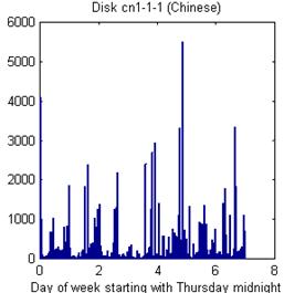
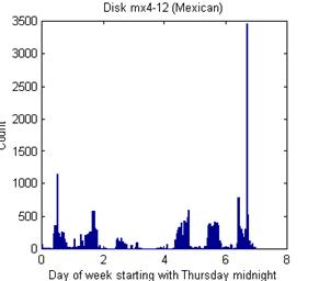
Figure 3: Histograms of modification times in week for two example disks.

Data also must be partitioned when it involves bursts, large numbers of file timestamps within the same short period.� Three kinds of bursts were observed: (1) one-time clusters such as those associated with installing new software, (2) clusters of periodic events within the week or the day, and (3) on-the-hour clusters apparently due to operating-system rounding.� Data of these clusters was removed from the main analysis file.� For the first kind, the criterion was more than 360 created files in a one-hour period; for the second, more than 50% of the total count of the week on any one day, or more than 30% in any one hour; for the third, 50 files created within five seconds of the top of the hour.� To help in identifying periodic patterns, clusters are removed from histograms by setting their counts to that of the average bin count for the histogram (since setting them to zero would create a �negative cluster�).� For example, a histogram of creation times over the days of the week of �6 2 10 152 8 500 313� was modified to �6 2 10 152 8 70.1 41.4�.

Our triage also identifies (but does not exclude from further analysis) those files with special relationships between their timestamps: files modified before being created, files accessed before being created, and files modified before being accessed.� Modification before creation is typical of purchased software, where the modification time originates from the vendor.� Access times before creation indicate files that have been accessed without changing the metadata, perhaps to reduce operating-system bookkeeping.� Modification before access (when modification is not before creation) indicates files that are probably read-only.

Triage took about one hour on the corpus.� Table 2 shows the results of analysis of the subsets resulting from this triage, indicating the file extensions, top-level directories, and bottom-level directories with anomalous counts for the subsets.� "Anomalous" was defined to mean that the difference between the set and its complement (opposite) was than 1.5 standard deviations greater than the expected value.

A related issue is to what extent files are created together on a disk, as when software or media files are downloaded together.� This was investigated by calculating the range of times in each nontrivial directory to see if they had any of the following characteristics, extending the ideas of [5]:

� All files in a directory have creation times within a minute.� This suggests they were downloaded or copied.

� All files in a directory have modification times within a minute.� This suggests they are used by automatic processes, such as log files.

� All files in a directory have access times within a minute.� This suggests they provide data used routinely such as initialization parameters.

� All files in a directory have modification times at least one day before creation times.� This suggests that the files were downloaded or copied from some other place that created them, as with applications software.

� All files in a directory have access times at least one minute after creation times.� This suggests that the files are frequently used, as with bookkeeping and log fil0es.

We checked for these conditions on the corpus of 1007 drives, but results were disappointing.� Of the 110,816 directories in the corpus, 158, 142, and 81 had time ranges within one minute for creation, modification, and access respectively.� 69 had only files modified before creation, and 16 had only files accessed after creation.� This suggests that time rounding to the hour by the operating system seriously affects the ability to detect grouped files from their times alone.

Table 2: Distinctive non-random features of important time-based subsets of the data.

Subset and count (from 5,643,824)	Distinctive extensions	Distinctive top-level directories	Distinctive immediate directories
Default time values (433,541)	Windows OS, help, executables	Windows OS	temporaries, Web
One-time creation clusters� (hours with > 360 count) (2,853,963)	none, audio, miscellaneous	root, Unix and Mac, miscellaneous	root, operating system
Periodic creation clusters in week (35,941)	Windows OS, links, executables, JPEG, audio	Documents and Settings, temporaries, miscellaneous	images
Access times on the hour (1,148,720)	graphics, JPEG, temporaries, Web, documents, Microsoft Office, links, integers	deleted files, Program Files, temporaries	operating system, images, Web
Modified only at creation (2,818,223)	none, graphics, JPEG, temporaries, Web, integers	root, deleted files, Documents and Settings, program Files	root, operating system, temporaries
Modified before creation (2,055,158)	Windows OS, documents, Microsoft Office, help, audio, program source, executables, XML, miscellaneous	deleted files, temporaries, Unix and Mac, miscellaneous	logs and backup, images, miscellaneous
Modified after creation (770,443)	Windows OS, Microsoft Office, links, help, audio, executables, miscellaneous	Windows OS	Web, miscellaneous
Accessed only at creation (906,413)	none, Web, links, XML, miscellaneous	Documents and Settings, Unix and Mac, miscellaneous	logs and backup, miscellaneous
Accessed before creation (1,729,401)	JPEG, temporaries, Web, documents, program source, XML, integers, miscellaneous	deleted files, temporaries, Unix and Mac	operating system, images, miscellaneous
Accessed after creation (3,008,010)	Windows OS, graphics, Microsoft Office, links, help, audio, executables	root, Windows OS, Program Files, miscellaneous	root, operating system, temporaries, Web
Accessed at modification (789,553)	none, Web, program source, XML	Documents and Settings, Unix and Mac	logs and backup, miscellaneous
Accessed before modification (2,014,228)	JPEG, temporaries, Web, program source, integers	deleted files, Windows OS, temporaries	operating system, images, miscellaneous
Accessed after modification (3,847,157)	Windows OS, documents, Microsoft Office, links, help, audio, executables, miscellaneous	root, Windows OS, Program Files, miscellaneous	root, operating systems, temporaries, images, Web
Non-default non-clustered times (591,818)	none, graphics, Web, documents, links, XML	Documents and Settings, Program Files, temporaries, miscellaneous	logs and backup, temporaries, Web, miscellaneous

We did a similar analysis on the file groups described in section II.B.� Figure 4 visualizes the sixteen time-related properties of the data after the normalization of section II.A following by application of the mapping �to get a number on the range of 0 to 1.� In Figure 4, redness is the normalized property value, blue is one minus the value, and green is one minus the absolute value of the difference between the red and blue values, so 0=blue, 0.5=light green, and 1=red.� Rows correspond to 30 groups of file extensions as described on the left, and columns correspond to the 16 time-related metrics described in section II.A that are listed below the image.

Figure 4: Visualization of differences in time properties of the 30 groups of file extensions.

C. Diurnal and weekly histogram patterns

One important way to categorize drives after triage is by their pattern of usage over the day and over the week.� This can be seen by taking histograms of times per each hour of the day and per each day of the week.� For this, creation times and most modification times were helpful.� Since most access times were rounded to the hour, they cannot be trusted to be meaningful except at coarse time scales.� Also excluded were modification times that occurred before creation times, as these suggested modifications by the software vendor, not by users who are the focus of this work.

The remaining histogram data shows distinct patterns, enabling a rough characterization of user types.� Figures 5 and 6 show example histograms for six disks after exclusion of default-time, erroneous-time, and bursty files.� Previous work [6] found that few of these disks had �more than one user, so their usage patterns usually correspond to the diurnal cycle of a single person or a business.� Such human activity patterns are well known [7].� The histograms were observed to fall into fourteen categories: (1) businesses active during the daytime; (2) businesses active during the evening; (3) businesses active in both day and evening; (4) businesses active during the night; (5) home users active on weekday nights and weekends; (6) users (either business or home) active every evening; (7) home users active on weekend days and evenings; (8) home users active during the night; (9) local business servers active during the day and evening; (10) local entertainment servers active during the day and evening; (11) �international� business servers active over all periods of day and night; (12) international entertainment servers; (13) usage that did not fit any of these patterns; and (14) little-used drives.

To classify usage, the method that worked the best was one of simplest, a nearest-neighbor case-based approach using just three parameters: (1) the ratio of rate of usage during weekdays to the rate of usage during weekends; (2) the ratio of the rate of usage during the day to the sum of all three rates of usage (day, evening, and night); and (3) the ratio of the rate of usage during the evening to the sum of all three rates of usage.� Note these were not the ratios of counts, but the ratios of rates, to adjust for unequal time spans.� Weekends were defined as Saturday and Sunday; day was defined as 0800 to 1700; evening as 1700 to 2400; and night as 0000 to 0800.� The ideal cases used are listed in Table 3.� The nearest-neighbor approach did not work well for drives with fewer than 25 files after removal of the default and bursty files as described above, which applied to 637 of the drives in the corpus; these were assigned to a �little-used� category.� Figures 5 and 6 show example disk distributions per day of the week and per hour of the day.� Disk 29 (from Canada) is a business user with traditional weekday-daytime hours of operation; disk 994 (from China) is a business operating in the evening; disk 403 (from Israel) is a home user of regular habits (note the sharp peak at 7PM); disk 695 (from Mexico) is a server local to one area of the world; and disk 855 (from Mexico) is a server that is more international in scope and entertainment-oriented judging by its use on weekends.

Figure 5: Usage per day of five disks.

Figure 6: Usage per hour of five disks.

Some drives were time-shifted by one to four hours from the ideal patterns.� These could be people with later or earlier schedules than most, or they could be misadjusted clocks [8].� All possible shifts of the hour histogram modulo 24 were examined to find the best match.� To prefer the smaller shifts in indifferent situations, the distance between ideal and actual histograms was multiplied by (1+0.1*|shift|) as a way to break ties well.� About 60% of the best shifts found on the test set were -1, 0, or +1 hours, and these could reflect errors in the setting or Daylight Savings Time offsets.� Note that shifts of more than four hours will be interpreted as different ideal profiles.

Histograms over hours and days can also be computed for subsets defined by the other three grouping attributes of file extension, top-level directory, and bottom-level directory.� Many matched best to the �day-evening business user� case that was the most common match for the drives.� Especially interesting were those categories which matched best to the �international server� case, like files with extensions of �jpg�, �wav�, �lrd�, �asx�, �sst�, and integers, and top-level directories of �Program Files�, �WINNT�, and �IMAGE�; these categories suggest automatically downloaded commercial products.� Also interesting were those which matched best to �home user� case such as files with extensions of �ram�, �chq�, �ima�, and �rdb�, and top-level directories of �MP 3�, �Otto�, �Ghost�, and �DDZ�, suggesting consumer-oriented software.

Table 3: Ideal ratios for cases of user periodic behavior.

Weekday ratio	Day ratio	Evening ratio	Case description	Inferred drive count in sample
0.8	0.8	0.0	business user	10
0.8	0.0	0.8	evening business user	51
0.8	0.45	0.45	day-evening business user	90
0.8	0.0	0.0	night business user	6
0.3	0.3	0.6	home user	24
0.3	0.8	0.2	day home user	3
0.2	0.45	0.45	day-evening home user	6
0.2	0.1	0.1	night home user	11
0.6	0.5	0.5	local business server	23
0.4	0.5	0.5	local entertainment server	7
0.6	0.33	0.33	international business server	86
0.4	0.33	0.33	international entertainment server	51
-	-	-	unusual	2
-	-	-	little used	637

Something else recognizable from a histogram is nonrandom patterns in the histogram counts values themselves, which suggest periodic scheduled use.� Consider the following histogram per hour over 24 hours of one disk:

78 26 108 30 20 16 24 16 10 12 10 0 2 4 36 30 52 90 64 138 82 40 104 72

7 of the 24 numbers are divisible by 10, and 10 of the 24 are divisible by 6.� These counts are significant, and suggest the machine is being updated every minute that is a multiple of 10 (suggesting 6 times per hour) or a multiple of 6 (suggesting 10 times per hour).� Extensions having histograms with these unusual features were �iqy�, �mdz�, and �bdr�, and� top-level directories with these were �System� and �Install�.� In general, the chance probability of a count of K with B bins and N items to distribute over those bins for small probabilities is approximately . �For N=24, B=10, and K=7, P is 0.0346; for N=24, B=6, and K=10, P is 0.0324.� Both these probabilities are sufficiently small for the above sequence to suggest a chance coincidence is unlikely.� In the sample drives, 9 had scheduling patterns every 10 minutes, and 5 had scheduling patterns every 6 minutes (of which 2 had both), with a 3% chance probability for each type.� As for exact matches in the counts per day of the week, two drives had an exact match on counts above 700, which was probably not due to chance.

IV. Comparison with times from Windows Registry

So far only directory metadata for a drive has been considered.� Useful times also appear in the log and registry records of events on systems [9].� Their time information is more complete than file-directory metadata for some files since it reports more than the last event of a type.� We took a sample of the registry data ("system hive") from 11 Windows XP disks in the corpus to see how their registry times correlated with those of the file times.� One measure of correlation is the fraction of registry times that occurred within an hour of some creation, modification, or access time of a file on the disk.� (An hour was selected to account for the observed rounding of times by the operating system).� Results varied considerably between disks (Table 4).� Correlations are also listed for just the modification times in the Windows operating system directories (like top-level directory Windows) because most of the matches were with files there, with some exceptions for program directories, and the best correlations occurred with modification times rather than creation or access times.

Table 4: Correlation of registry times with file times on 11 example disks.

Drive number	#32	#82	#92	#120	#125	#284	#535	#689	#737	#755	#757
Number of registry times	6149	5328	3332	6282	16118	7864	7562	2998	3954	7351	8459
Correlation with creation time	.009	.123	.000	.000	.144	.000	.060	.000	.190	.039	.143
Correlation with modification time	.010	.653	.000	.002	.158	.000	.077	.000	.190	.039	.178
Correlation with access time	.000	.105	.000	.000	.087	.005	.026	.000	.499	.132	.032
Correlation with modification time of only Windows OS files	.008	.576	.000	.000	.131	.000	.035	.000	.190	.039	.131

�

Registry times were more bursty than file times, which is not surprising since they report important changes to the operating system.� Figure 7 shows a typical example in the data from disk #757 compared with the corresponding disk modification times.� 9 of the 11 disks like this one showed an earliest peak of registry times that was considerably larger than the other peaks, and which appears to represent the installation and setup of the drive.� In addition, the peaks at the end of registry times for drive 757 probably represents the decommissioning of the drive prior to sale to us.� Identification of these starting and closing activities is important, as it allows us to calculate a usage interval and usage rates for a drive.

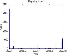
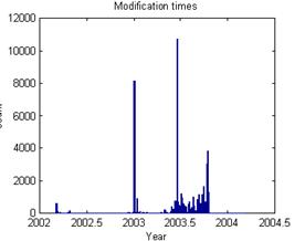
Figure 7: Registry times versus file modification times for an example disk.

V. Analysis of sampled data

Our experiments required a full scan of a drive image to extract all file data.� An important question is to what extent a sample of the drive image will suffice for adequate analysis in a hurry.� If the sample is done randomly and has a sufficient size, many of the statistical methods explored here will be effective.� Reliability of statistics of random samples is a well-studied problem.� The �formula for the variance of a parameter in a sample of size n from a population of size N with variance �in the parameter applies to the statistics on file subsets that are described in this paper.� For statistics that are fractions of mean value p, .

Default time values and some clusters can be identified in a sample.� However, sampling makes it harder to find clusters since these require sufficient counts above the random background rate to notice.� Unfortunately, little correlation was found between the times of clusters of different drives.� These appear to be controlled by login times, which vary between drives.� So sampled data is more likely to be confounded by the occurrence of unrecognized clusters.

VI. Related work

Despite the widespread use of file timestamps to create timelines within the forensics community, there have been surprisingly few efforts at using this information to cluster files.� [10] introduced this approach.� However their purpose was to use outliers to identify suspicious files that might result from a break-in, not to understand the pattern of files on a drive.� More broadly, [11] analyzed file systems from 4801 desktop PCs running Windows at Microsoft Corporation, and were able to model file sizes, ages, lifetimes, directory sizes and directory depths using classical distribution functions.� This experiment was repeated every year for five years and resulted in a �generative model that explains the namespace structure and the distribution of directory sizes� [12].� Reference [13] studied methods on DZero to cluster files for improving scientific workload.

VII. Conclusions and future work

As the first step towards building a system that can automatically classify the usage patterns on a hard drive, this work explored timestamps associated with files.� Many distinctive diurnal and weekly patterns are apparent with simple analysis.� But separate consideration of files with timestamps that were default values or which appeared in large bursts was essential.� Clustering of the files based on extension and directories was very helpful in understanding the distinctive characteristics of different kinds of files based on their timestamps, and will be explored further in our future work.

The Windows Registry also has timestamps, and it was observed that these timestamps are not well correlated with the timestamps on files.� This is actually encouraging, as it means that registry data will likely complement file data for drive classification.� Future work will extend these comparisons to log and audit records�� This preliminary study also predominantly examined examples of the Windows operating system and some flash-based storage devices, and it would be useful to review other operating systems and media for careful comparisons.�

Acknowledgements

The views expressed are those of the authors and do not necessarily reflect those of the U.S. Government.� Joshua Gross and Andrew Schein assisted us in the collection of registry timestamps.� We would like to thank Vassily Roussev for his helpful comments on this paper.�

References

[1] N.� Rowe, "Measuring the effectiveness of honeypot counter-counterdeception," Proc. Hawaii International Conference on Systems Sciences, Koloa, Hawaii, January 2006.

[2] S.� Garfinkel, P.� Farrell, V.� Roussev, and G.� Dinolt, "Bringing science to digital forensics with standardized forensic corpora," Digital Investigation, Vol.� 6, S2-S11, 2009.

[3] S.� Garfinkel, "Automating disk forensic processing with SleuthKit, XML and Python," Proc. Systematic Approaches to Digital Forensics Engineering, Oakland, CA, 2009.

[4] J.� Olsson, and M.� Boldt, "Computer forensic timeline visualization tool.," Digital Investigation, Vol.� 6, S78-S87, 2009.

[5] K.� Chow, F.� Law, M.� Kwan, and P.� Lai, "The rules of time on NTFS file systems," Proc. 2nd International Workshop on Systematic Approaches to Digital Forensic Engineering, Seattle, Washington, April 2007.

[6] S.� Garfinkel, A. Parker-Wood, D. Huynh, J. Cowan-Sharp, and J. Migletz, "A solution to the multi-user carved data ascription problem," draft, October 2009.

[7] R.� Refinetti, Circadian Physiology, 2nd Edition.� Boca Raton, FL: CRC Press, 2005.

[8] F.� Buchholz and B.� Tjaden, "A brief study of time," Digital Investigation, Vol.� 4S, 531-542, 2007.

[9] Y.� Zhu, P.� Gladyshev, and J.� James, "Temporal analysis of Windows MRU registry keys," in G.� Peterson and S.� Shenoi (Eds.), Advances in Digital Forensics V, IFIP AICT 306, pp.� 83-93, 2009.

[10] B.� Carrier and E.� H.� Spafford, "Automated digital evidence target definition using outlier analysis and existing evidence," Proc. Fifth Digital Forensic Research Workshop, 2005.

[11] J.� Douceur and W.� Bolosky, "A large-scale study of file-system contents," Proc. SIGMETRICS �99, Atlanta, GA, 1999.

[12] N.� Agrawal, W.� Bolosky, J.� Douceur and J.� Lorch, "A five-year study of file-system metadata," ACM Transactions on Storage, Vol.� 3, No.� 3, Article 9, October 2007.�

[13] S.� Doraimani and A.� Iamnitchi, "File grouping for scientific data management: lessons from experimenting with real traces," Proc. HPDC�08, Boston, MA, 2008.