Abstract�Simulations can produce large quantities
of data.� To reason about the results of simulations, machine-learning methods
can be helpful.� We explored a case-based reasoning approach to summarizing the
results of a probabilistic simulation of naval combat involving missiles.� We
used a tree structure to index the data and showed that it gave good accuracy
in estimating the results of this simulation with new parameters.� We are now
extending these ideas to a more complex military simulation.
Keywords�simulation, case-based reasoning, model, results,
trees, interpolation, salvo
This paper appeared in the Proc. Intl. Conf. on Computational
Science and Computational Intelligence, Las Vegas, NV, USA, December 2019.
I.
Introduction
Case-based reasoning is a machine-learning method based
on comparing current inputs to past inputs [1].� It requires an indexing scheme
to find the most similar cases to a current case, often accomplished by a
multi-attribute tree.� Unknown characteristics of the current cases can be
inferred from the average of the similar cases.� When cases are plans, this is
called �case-based plan adaptation� [2].� For simulation applications, stored
results of previous simulation runs can be compared to a current situation to get
a set of predictions of likely outcomes that can be averaged in some way.�
Weights on attributes for distance calculations can be either be obtained from
human experts or by training from the results of simulations. �
Case-based reasoning provides a simpler alternative to
artificial neural networks for summarizing the results of simulations that has
the advantage of requiring much less training effort.� It can also perform well
with small amounts of training data, unlike neural networks which in their deep
forms requires millions or billions of training cases to perform well.� This
also means it can perform better than neural networks on time-critical
decisions when data is streaming in quickly.� These issues are important for
military planning, since data from exercises and actual conflict that could be
used for training the system are expensive and not numerous, and tasks are
often time-critical.� Case-based ideas can be used in several ways for military
planning.� They can be used to find the best of several detailed engagement
models that apply to a given situation; many militaries have detailed models of
the effects of their weapons.� They can be used to find good assignments of
weapons to targets.� They can also be used to find full mission plans from
similar previous situations.� The last is what we focus on here.
II. Data farming approach
This work used data from a �salvo� simulation of naval
combat produced by Tom Lucas and Susan Sanchez, which is similar to some others
such as the South Korean military planning system of [3] for land combat.� The
salvo model is a modified version of a standard naval model developed
originally by [4] and refined by others.� The version by Lucas and Sanchez was
designed specifically to model missile exchanges.� It did lack some important features
of naval combat such as readiness, aircraft factors, distance between
adversaries, and mission requirements which we are addressing currently as
described in section IV.
Our goal was to use results from the salvo simulation to
build a predictive model, a �data farming� approach [5] which has been used
successfully for many military-planning problems [6].� The salvo simulation has
only 26 parameters, but that still provides a sufficiently large variety of inputs
that design of a good data structure to index and store the results of runs is
important.� Simulation inputs can be represented as 26-element vectors.� We
generated 100,000 random vectors and ran them through the simulation to
generate outputs.� Four metrics �were obtained for each run of the average and
standard deviation of its duration, and the average and standard deviation of
the ratio of the losses of on the two sides from the engagement.� A logarithm
was applied to durations to better achieve a normal distribution.� For the loss
ratios, we used the formula  , which can
be simplified to
  . �Blue�
represents friendly forces and �red� represents adversary forces.� The �s� or
sigmoid function is needed to model the relative indistinguishability of high
and low ratios; it models that realization that it is not much different if we
have destroyed 100 times more versus 200 times more of an adversary than they
destroy of us.
III. Case-based reasoning approach
Case-based reasoning uses four steps, which have been called
retrieve, reuse, revise, and retain [7].� We use a tree for retrieval of data
of the most-similar input vectors.� Reuse will be accomplished by taking a
weighted average of outputs of the most similar cases.�� Revising is unnecessary
to our application because the reuse method is not complex.� Retaining can be
done once a proposed new set of input parameters is run through the simulator
to confirm its predicted outcome; in fact, retained cases will be more useful
than random cases because they are come from real needs.
A. �Building an
index tree to the cases
For our military task, it is important to find similar
cases quickly, and an index tree is a good way.� The 100,000 simulation results
were indexed with a tree with a branching factor of 10.� This was accomplished
by dividing the range of each input parameter into 10 bins by sorting the values
and finding the 10th, 20th, �, and 90th
percentiles.� Preliminary experiments were conducted to confirm that 10 was a
good number of bins.� The means there were  �sets of input
parameters, so this space will be sparsely populated compared to the
  �items of run
data. �The tree is useful in finding similar cases; then, because the salvo
model is based on smoothly-varying parameters and equations, interpolation is
effective for predicting results on new cases.
Building the tree is simplified when some input
parameters have significantly less effects on results and can be mostly
ignored.� These were found by computing linear regressions on output metrics as
a function of the 26 parameters.� We did four regressions on the four output
metrics: the mean loss ratio, the standard deviation of the loss ratio, the
mean of the log of the duration in number of exchanges, and the standard
deviation of the duration in numbers of exchanges.� Results are shown in Table
1.� The magnitude of the coefficients reflects their effect on the target value.�
So the ten most important inputs based on mean loss ratio, our most important
output, were b_off_miss_salvo_size, r_ship_surv, r_off_miss_salvo_size,
b_ship_surv, b_n_ships, r_def_miss_salvo_size, r_n_ships,
b_def_miss_salvo_size, b_decoys_surv, and r_decoys_surv.�
We used the most significant factors for the loss ratio
to build the index tree that maps from some new set of inputs to estimates of
the four metrics.� The attributes used were the most significant factors in
decreasing order of significance according to Table 1 as one descends the
tree.� To build the tree top-down, at each level we computed means and standard
deviations of the loss ratio for each of the ten bins of the attribute assigned
to that level, and added nodes to the tree when the standard deviation of the
cases that apply exceeded a fixed threshold.� Otherwise, the node of the tree
became a leaf node and we stored the means of the four metrics there for the
cases that applied to it.� Because bins were defined by percentiles on overall
distributions of the parameters, subtrees tended to be balanced except when
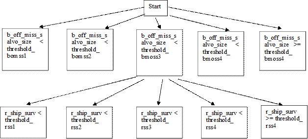
inputs were strongly correlated.� Figure 1 shows part of two levels of an
example index tree showing five nodes on the first level and five nodes on the
second level.
B. Reusing cases
Reuse of our case library means finding the most similar
cases to some new situation.� Our index tree is a form of �hierarchical
retrieval� in the terminology of case-based planning of [3].� Since a plan
for our problem is a set of numeric allocations, plan reuse will be
�transformational� rather than �deviational� in the terminology of [2] and will
modify parameters of existing cases rather than generalize from them.
To retrieve an output estimate from
the tree for a new set of input parameters, we first compute the bins for those
parameters.� We then traverse the tree until we get to a leaf node for that set
of bins, and use the estimates stored at that leaf node since the leaf nodes
are usually where the standard deviation is below a specified minimum.� Leaf
nodes could be above the minimum when the number of cases used to build the
tree is insufficient, but we did not find this to be a problem for our
simulation and 100,000 cases.� If we need higher accuracy in the estimate at a
leaf node, we can take a weighted average with neighbor bins as well, and this
is desirable when the metrics vary considerably with parameters.� We do this by
looking up all sets of parameters within K bin numbers of the target set of
parameters and averaging their metrics.� Since 10 bins were created for each
attribute range, a variation of 1 in each bin number should have roughly the
same effect on the inputs.� So given a set of inputs to lookup, we can first
try to look up those inputs in the index, then all 52 neighbors differing by
only one bin number, then all 52*52 neighbors differing by two bins numbers or
twice on one bin number, and so on.� We use the average of what we have found
as our estimate of the metric.
An important question is how deep the tree should be to
get sufficiently good estimation performance.� Table 1 showed that only about
10 factors are important in determining performance, so we do not need to go
deeper than 10 with our simulation data.� We also studied this experimentally
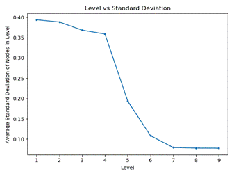
by measuring the average standard deviation of the loss ratio mean as a
function of level in the tree.� Figure 2 shows results for a subset of
simulation runs numbering 34,000.� As we descend in the tree and specify ranges
on the input parameters, the standard deviation of the loss ratio should
decrease for the more restricted situations.� However, it is interesting there
is a sharp decline starting with 4 inputs, which shows that the first four
inputs are the most critical to performance.� This is probably related to the
fact a balanced tree for 34,000 items should have a depth of the logarithm to
the base 10 of 34,000, which is 4.53, and our trees are close to balanced. �However,
the Figure indicates less than perfect balance, and to err on the side of
safety, we built trees of depth 7 for the index in our experiments.� Note that Figure
2 levels off at 0.05 rather than 0 at depths 7-9 because we do not continue the
tree if the standard deviation of the loss ratio is less than a threshold.

Figure
2: Average standard deviation of loss ratio as a function of number of levels
deep in the tree, for a tree built from 34,000 runs of the simulation.
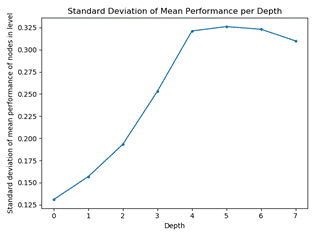
On the other hand, the standard deviation of the mean
loss ratio increases with level as the tree becomes better able to approximate
a wide variety of situations (Figure 3).� Since the loss ratio ranges between 0
and 1, and a uniform random distribution has a standard deviation of  , performance
leveled off near where it would be with a uniform random distribution.� That
suggests that the simulation was capable producing a wide evenly-spaced set of
loss ratios.
C. Implementation
efficiency
We measured time to generate the tree and to use it on a
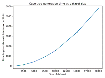
six-year-old Windows workstation.� Results are shown in Table 2.� As expected,
generation time was an exponential function of the number of simulation runs
used to build it �(Figure 4) though its concavity (second derivative) was mild.�
After the tree has been generated, it can be saved to disk and
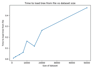
reloaded in significantly less time than the time to create it (Figure 5).

Figure
3: Standard deviation of the mean loss ratio as a function of depth in the
index tree.
Table 2: Timings on the
index tree as a function of the number of simulations.
|
Number of simulation records
|
Time to generate tree, maximum depth of 7 (seconds)
|
Time to generate list (seconds)
|
|
1000
|
18.31
|
0.01
|
|
2500
|
104.76
|
0.04
|
|
5000
|
407.96
|
0.08
|
|
7500
|
901.64
|
0.13
|
|
10000
|
1447.69
|
0.13
|
|
15000
|
3658.46
|
0.24
|
|
20000
|
6123.10
|
0.25
|
|
50000
|
30996.77
|
0.74
|

Figure
4: Time to generate the tree as a function of the number of simulation runs to
index.
Retrieval time was tested by randomly generating simulation
parameters 500 times and averaging the performance. �With  �possibilities,
random cases rarely had the same bin assignments used to create the tree, yet
the extra time to retrieve estimates for them was not significant.� Worst-case
retrieval time should remain constant as it is determined by the depth of the
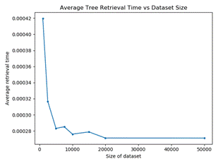
tree. �However, we found an unexpected decrease in retrieval time as the size
of the dataset (number of simulation runs) grew (Figure 6). �We suspect that as
the case base grows, it is easier to find input clusters with a sufficiently low
standard deviation to enable pruning of the tree.

Figure
5: Time to load pre-generated tree as a function of number of simulation runs.

Figure
6: Average retrieval time versus number of simulations stored in the index
tree.
We also compared the accuracy of the tree�s predictions to
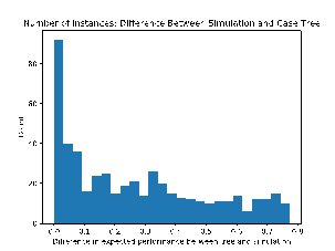
those obtained by running the simulation (Figure 7).� As the salvo model itself
has random variation, its results could significantly differ between runs, so we
averaged results over 10 runs to get data for the tree.� Interestingly, the
larger errors tended to be non-normal and evenly distributed on a range of 0.10
to 0.75.�� That suggests that our simulation exhibits a phase-change phenomenon
in which small differences in inputs can lead to very different outcomes.� But
other simulations may differ.
D. Linear
combinations to add flexibility to reuse of cases
An alternate way to use cases to predict results for new
inputs is to store plans only for simpler tasks, and then combine them to get
plans for more complex tasks, as a form of �transformational� plan reuse [2].�
This is useful when we do not have many cases, as when they have been generated
by simulations controlled by human players.� Many wargames have this
characteristic as it is costly and time-consuming to run realistic wargames
with human players.

Figure
7: Distribution of error between predicted loss ratio using the tree index and
the results of a single simulation run on the same parameters.
One way to combine cases is to separately develop plans
for each of a set of quite different cases, then add the numbers of the plans
into one overall plan vector with an estimated performance based on the
weighted sum of the performances of the individual plans.� This approach is
inspired by the use of basis vectors for matrices.� The plans combined will
need to be scaled as necessary to fit available resources.� For instance, if we
have 100 weapons of type 1 and 50 weapons of type 2, we could map to a case
with 50 weapons of type 1 and 25 weapons of type 2 by multiplying parameters by
0.5.� However, decreasing the size of inputs from what was previously tested may
increase the standard deviation of the result.� Note for this to work, plans
must scale assets of both sides.
Suppose we have N attributes and M models that are
similar to the current situation as represented as an N-element vector whose
attribute values are  .� Suppose
model j has attribute values
  .� Suppose we
will take a linear weighted average of the M models in the form of
  �where
  �is the
vector of attributes.� We want to find the
  �that will
minimize the error.� A classic approach is to minimize the least-squares error
  .� Since
  , setting
that to zero results in a set of M linear equations for each j in M unknowns in
the form
  �which are
straightforward to solve.
Choosing the M cases for reuse can be done by heuristic
search using as a fitness function the total least-squares error.� We can start
with M=1, then M=2, etc. until improvements in the error are not significant or
M reaches a reasonable maximum.� However, estimate accuracy will suffer for
larger M, and it may be a good idea to limit M to 1 or 2.� With M=1, the least-squares
fit is  .� With M=2,
the fit is
  �and
�and  �where�
  ,
,  ,
,  , and
, and  .� An M=2 fit
would be good when combining simulations of two dissimilar allocations that
have been tested separately.� For our military applications, that could be
dissimilar weapons.� For example, suppose there are only three parameters whose
values for a new situation are (50,50,80) for three types of weapons, and we
can match it to two cases of (100,50,0) and (0,30,100).� Then
  �and
�and  .� If the
average loss ratio for the first case was 0.8 and the second was 0.6, the
estimated loss ratio will be 0.504*0.8 + 0.802*0.6 = 0.733, using the classic
formulation for data fusion of two independent distribution.� The associated
standard deviation is
  .
.
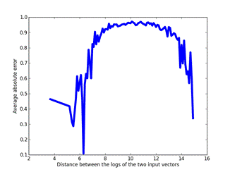
Figure 8 shows the results of 2000 experiments where we
chose two random input vectors previously run through the simulation, computed
the geometric mean of the vector components, and computed the error between the
average loss ratio of simulation runs on that average and the average loss
ratio of the averaged loss ratios of the two vectors.� The weighting was done
using the computed  �and
�and  �described
above; distance was computed using the logarithms of the ratios of one plus the
counts to be relatively consistent with the geometric mean while handling zero
counts.� It can be seen in the Figure that this two-point averaging only gets a
good result for distances less than 7, a distance that should be achievable for
a tree of 100,000 nodes for our salvo model.� For this threshold, the average
error for the two-point estimate was 0.103 whereas the average error of the
tree estimate was 0.129, with standard deviations of 0700 and 0.641
respectively.� Even though the mean was a little better for the two-point
estimate, the large standard deviations do not inspire confidence in its
estimates and suggest that the approach described in sections III.A and III.B is
sufficient in most cases as well as being faster.
� 
Figure
8: Error using the two-vector approximation of the simulation loss ratio versus
the actual simulation result.
IV. Application to real military
planning
This work tested a method of planning of naval missile
strikes intended for the BREM project.� Simulations and exercises can provide
the input similar to that of our experiments described above with the salvo
model.� BREM has significantly more numeric input parameters than the salvo
model, around 300.� They include sensors broken down by type and player; weapons
broken down by type, player, and round; defensive capabilities broken down by
target, weapon, and player; degree of intelligence about the adversary broken
down by type and player; readiness broken down by activity, player, and
weapon/aircraft/personnel/training; electronic and cyber offensive
capabilities; and weather and sea-state conditions.
Until we can do a regression fit on sample runs, it is
hard to say which factors are the most important, or predict how deep the tree
needs to be.� We assume from our earlier experiments that 10 bins for each
parameter will be effective.� Since an upper bound on the number of leaf nodes for
such a tree is  for N levels,
an upper bound on the number of nodes total in the tree is�
  .� Thus a
tree of depth 10 will require about 1000 times more nodes than a tree of depth
7.� However, actual size will depend on the threshold on maximum standard
deviation and the number of simulation runs whose data is entered into the
tree.� A useful strategy for reducing workload would be to aggregate some of
the factors into composites to reduce the size of the tree.� We could, for
instance, aggregate counts of weapons into a single total, or aggregate
communications, electronic-warfare, networking, and sensors under the title of �equipment�.
V. Conclusions
We have shown that a relatively simple case-based
approach can be used to summarize results in a tree structure of simulation
runs of a complex model.� The tree can be used for lookup directly, or results
of several lookups can be averaged to get greater accuracy.� Results on testing
a 26-parameter simulation were promising, although the stochastic nature of the
simulation meant the tree prediction could have errors.� This approach should
provide a useful simpler alternative to training of neural networks as it is
cost-effective with relatively small amounts of simulation data.
Acknowledgements
This work was supported by ONR through Bruce Nagy at NAWC-WD
China Lake.� Thanks to Paul Sanchez for the salvo model.� The opinions
expressed are those of the authors and do not represent those of the U.S.
Government.
References
[1]
I. Witten, E. Frank, M. Pal, and C. Hall, Data Mining: Practical Machine
Learning Tools and Techniques,� fourth edition, Morgan Kaufmann, 2016.
[2] H. Munoz-Avila and M.
Cox, �Case-based plan adaptation: An analysis and review,�� IEEE Intelligent
Systems, July/August 2008, pp. 75-81, 2008.
[3] W. Kim, S. Baik, S.
Kwon, C. Han, C. Hong, and J. Kim, �Real-time strategy generation system using
case-based reasoning.� Intl. Symposium on Computer, Consumer, and Control, pp.
1159-1162, 2014.
[4] W. Hughes, �A salvo
model of warships in missile combat used to evaluate their staying power,� Naval
Research Logistics, Vol. 42, No. 2, pp. 267-289, 1995.
[5] S. Sanchez, P. Sanchez,
P., and H. Wan, �Simulation experiments: Better insights by design,� Proc.
Summer Simulation Multiconference, Paper 53, 2014.
[6] D. Kallfass and T. Schlaak,,
�NATO MSG-088 case study results to demonstrate the benefit of using data
farming for military decision support,�� Proc. Winter Simulation Conference,
Berlin, DE, December 2012.
[7] D. Borrajo, A. �Roubickova,
A., and I. Serina, �Progress in case-based planning,� ACM Computing Surveys,
Vol. 47, No. 2, Article 35, January 2015.
![]() , which can
be simplified to
, which can
be simplified to ![]() . �Blue�
represents friendly forces and �red� represents adversary forces.� The �s� or
sigmoid function is needed to model the relative indistinguishability of high
and low ratios; it models that realization that it is not much different if we
have destroyed 100 times more versus 200 times more of an adversary than they
destroy of us.
. �Blue�
represents friendly forces and �red� represents adversary forces.� The �s� or
sigmoid function is needed to model the relative indistinguishability of high
and low ratios; it models that realization that it is not much different if we
have destroyed 100 times more versus 200 times more of an adversary than they
destroy of us.![]() �sets of input
parameters, so this space will be sparsely populated compared to the
�sets of input
parameters, so this space will be sparsely populated compared to the ![]() �items of run
data. �The tree is useful in finding similar cases; then, because the salvo
model is based on smoothly-varying parameters and equations, interpolation is
effective for predicting results on new cases.
�items of run
data. �The tree is useful in finding similar cases; then, because the salvo
model is based on smoothly-varying parameters and equations, interpolation is
effective for predicting results on new cases.