Approved for public release;
distribution is unlimited
Interpreting Suspicious and Coordinated Behavior in a Sensor Field
August 2008
Neil C. Rowe
U.S. Naval Postgraduate School
Code CS/Rp, Monterey, CA 93943
ABSTRACT
We report on recent work we have done on detection of two kinds of militarily interesting behavior in an urban battlespace, detection of suspicious behavior and detection and classification of coordinated movements of groups of people.� The first is important in detecting terrorism and IED emplacement, and the second is important in detecting military adversaries and what they are doing.� Our approaches use only "pose" information, the locations and orientations of people within the sensor field, as extracted from tracking by a fusion of various nonimaging sensing modalities.� Restriction to nonimaging sensors saves money, and restriction to pose information avoids most of the serious privacy concerns.� We first explain our approach to tracking using signal strengths alone.� From experiments with both staged and nonstaged behavior in a public area, we found that the most useful clue to suspicious behavior was the norm of the acceleration vector averaged over several different time scales.� With detection and classification of groups of people, by contrast, no single metric was as good as combinations of metrics.� We are exploring a variety including average distances between people, uniformity of distances, linearity of the positions of people, number of clusters of people, number of directions in which they can see, overall visibility, average speed of the group, and uniformity of the speed of the group.� A key challenge is to make these metrics scale-free as with the acceleration vector analysis.
This paper appeared in the Proceedings of the Meeting of the Military Sensing Symposium Specialty Group on Battlespace Acoustic and Seismic Sensing, Magnetic and Electric Field Sensors, Laurel, MD, August 2008.
1. Introduction
Detection of suspicious and other interesting behavior is a challenging problem.� Video surveillance by personnel is tedious and prone to errors (Hackwood and Potter, 1998).� Automated video surveillance would seem promising, but it has encountered a number of technical challenges (Valera and Valestin, 2005).� Determining exactly what people are doing can be challenging.
We are exploring an approach that looks only at pose information for people, their position and orientation.� This does not require understanding posture, gait, and other sophisticated features which are more difficult to extract from images.� It entails far fewer concerns about violation of privacy since faces need not be analyzed.� We think we can gain sufficiently useful information from just pose that we can direct human security personnel to area to find for themselves what is going on.
Such information can be obtained from relatively simple sensors such as magnetic, passive-infrared, seismic, or acoustic.� Our research team has been exploring such sensors for the last few years (Sundram, Poh, Rowe, and Singh, 2008) using a testbed of Crossbow sensors in a public area at our school.� Currently we are focusing on detecting behavior that could be associated with emplacement of improvised explosive devices (IEDs) for use in homeland security and peacekeeping operations.
This paper will survey three parts of our research. to analyzing the data provided by sensor networks� First, we describe work on tracking objects with simulated sensor grids, and algorithms we have developed based on signal strengths alone.� Second, we describe work we did on assessing simple clues for suspicious behavior in video with experiments including some deliberately staged behaviors.� Third, we describe work we have done on assessing the consistency, cohesion, visibility, and other metrics on groups of people towards determining when they are more likely to engage in suspicious behavior.
2. Simulation of tracking with simple sensors
Setting up experiments with the Crossbow sensors is time-consuming, and many environmental factors can affect the results.� So we built a simple simulator of them to run experiments.� In particular, we used it to explore how complex behaviors affect tracking success using standard tracking algorithms, an important issue not much addressed in previous research.� While the Crossbow sensors have some directional characteristics, these are variable and hard to model.� So our initial work has focused on tracking with just signal-strength information.
We simulated a rectangular grid of sensors detecting sources moving across their field.� Signal strength was assumed to be the sum of signals detected from all sources, where the strength of each signal was i/(m+d)^2, where i is the intensity of the source, d the distance from the source to the sensor, and m the minimum radius from the source.� The inverse square law is a good model for many sensing modalities since, with many wave and field phenomena, signal strength is proportional to the area of a sphere centered at the source and touching the sensor; it is particularly good for modeling magnetic, acoustic, and seismic sensors.� We assume the sensor field is placed in a small unobstructed area like a public square, so that determination of signal strength of reference signals at each sensor is not necessary as in (Zarimpas et al, 2005) Enforcement of a minimum distance is necessary to avoid unstable behavior with very-near sources.
Our simulator creates object tracks in the sensor space and calculates the associated signal strengths to provide test cases for analysis.� Analysis then tries to reverse the process and infer the source locations from the strength patterns.� Work addressing a similar problem of triangulation on signal strengths with different techniques is (Figueiras, Schwefel, and Kovacs, 2005).
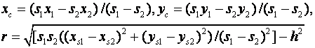
One approach is to do an optimization similar to that done for GPS localization (Kaplan et al, 2005).� A starting state is to infer that each peak of signal strength in the sensor grid is next to a source. ��We then adjust the locations of the inferred sources using the partial derivatives of the error defined as:

We can use these components to do gradient descent to find the positions and signal strengths that minimize the error of the readings.� Since we want a minimum, we should travel in the opposite sign of the partial derivatives of C, and since we can adjust the step size by feedback, we need only use the ratios of the components to determine direction.� Hence we can define a gradient direction by:

Unfortunately, these equations are tricky to use for real sensor networks since the optimization space has many local minima.� Thus convergence is a problem if the initial estimates of the tracked objects are not close to their actual locations.� In experiments with an average of two random constant-speed tracks across a 3 by 3 sensor array in the form of a square grid, convergence failed 86 out of 110 times when assigning sources initially to the local maxima of the signal in the sensor grid.
We got better performance by using a ratio of signal strengths in a variation on the approach of (Lee et al, 2006).� If we assume that the observed signal strength is due only to each sensor�s nearest source (we can subtract out the estimated effect of other sources otherwise), we have for two sensors at the same instant the same source strength, and hence:
![]()
This gives an equation of a circle for the locus of points on which the sensor could lie.� The center and radius of this circle are:
We can thus intersect two circles (from three sensors) to reduce the locus of two points.� With more than three sensors, we can find the "consensus center" by finding the set of all intersection points and repeatedly removing the furthest point from the centroid of the set until we have two points of which to take the centroid.� Once we have inferred the source points, we can compute their signal strengths, then recompute the positions and strengths iteratively until accuracy is sufficiently good.� Note, however, that the problem is ill-conditioned if the signal strengths are close to one another.
For this method of estimation track locations to work we must be careful to choose readings of signal strength from at least four sensor nodes including the local maximum, which gives us three circles to intersect.� It is also important to obtain at least three different horizontal and three different vertical values in the sensor readings to avoid the ill-conditioning problem.� We thus chose the four horizontal and vertical neighbors for each sensor in the square sensor grid, except along borders of the grid where used points deeper within the grid to obtain three along each dimension.� This gives five sensor readings and six circles to intersect.
Note that this approach is well suited to local computation on the sensor grid since we only need to bring together data from five neighboring sensors.� Eventually, however, the tracking results must be forwarded to a database node.� It also does not require a perfectly rectangular grid as long as sensor positions are known in advance.
We ran our simulation to obtain upper bounds on performance of a real sensor network.� Table 1 presents some example results for a 100 by 100 grid over a time interval of 20 seconds, averaged over 100 runs for each entry.� A square frame around the sensors was constructed whose distance from the nearest sensors was the same as the distance between neighbor sensors; random starting and ending locations were chosen on the edges of the frame.� Random starting times were chosen in the 20-second interval, but tracks could continue after 20 seconds as necessary to reach their goal points, and the results covered this extra time.� The average velocity per unit of the track was 10 and the average strength was 5 in all these experiments.� "V sd" the standard deviation of that velocity for the track (for variation perceived by all sensors), "s sd" the standard deviation of that strength (for variation perceived by all sensors), "si sd" is the standard deviation of the observed strength at each sensor for a signal of fixed strength, and "h dev" the average random deviation in radians of the track heading from the ideal heading towards its goal point (to model wandering).� "Tracks" means how many different tracks were created during the time interval.� The two numbers for each entry represent the average distance error in the track position and average error in the logarithm of the strength of the track at that position.
It can be seen that our circular optimization definitely improves the estimate of track positions, even with 8 tracks where it can more easily get confused by the multiple signal sources.� Doing it more than once does not help (despite its need to guess locations of far tracks).� Doing a subsequent optimization using the gradient formulas shown above actually worsens performance considerably on the average, illustrating how ill-conditioned the problem is.� Varying the average velocity and signal strength of the tracks and their variance had little effect on performance.� However, increasing the error with which individual sensors perceived the same signal did naturally degrade performance; just a 40% error in perceived signal strength made circle optimization significantly less effective for improving track-location estimates, though not so much on improving signal-strength estimates.� However, performance was not degraded as much as the introduced error, suggesting that the sensor consensus helps reduce errors.� Bounding of this latter error will be the principal focus of future experiments with our real-world sensor network.
These tracking methods did not exploit velocity consistency between different time intervals as is important in applications like radar tracking of aircraft.� Such methods could significantly improve our tracking performance.� However, we want to detect suspicious behavior, and as we will explain in the next section, accurate detection of sudden accelerations is critical for this.� If we were to seek more velocity consistency in tracking, we would dilute these key acceleration phenomena.
Table 1: Simulation results for straight tracks across a square sensor grid.
|
|
grid |
v sd |
s sd |
si sd |
h dev |
1 track |
2 tracks |
4 tracks |
8 tracks |
|
Track locations are signal peaks |
10x10 |
0 |
0 |
0 |
0 |
1.826, 0.324 |
3.189, 0.541 |
5.738, 0.955 |
10.935, 1.544 |
|
Track locations from circle estimation |
10x10 |
0 |
0 |
0 |
0 |
0.000, 0.000 |
0.369, 0.026 |
1.378, 0.108 |
6.042, 0.447 |
|
Same |
10x10 |
5 |
2.5 |
0 |
0.3 |
0.000, 0.000 |
0.278, 0.021 |
1.217, 0.102 |
5.186, 0.437 |
|
Same, estimation done twice |
10x10 |
5 |
2.5 |
0 |
0.3 |
0.000, 0.000 |
0.278, 0.024 |
1.217, 0.114 |
5.186, 0.459 |
|
Same, estimation then traditional optimization |
10x10 |
5 |
2.5 |
0 |
0.3 |
0.000, 0.000 |
1.926, 0.020 |
9.093, 0.189 |
24.698, 0.959 |
|
Same, circle estimation |
4x4 |
5 |
2.5 |
0 |
0.3 |
0.000, 0.000 |
1.841, 0.063 |
9.275, 0.309 |
28.292, 1.094 |
|
Track locations are signal peaks |
10x10 |
5 |
2.5 |
2 |
0.3 |
1.851, 0.324 |
3.042, 0.521 |
5.411, 0.869 |
10.551, 1.472 |
|
Same, circle estimation |
10x10 |
5 |
2.5 |
2 |
0.3 |
0.805, 0.059 |
1.563, 0.108 |
3.109, 0.216 |
7.405, 0.538 |
3. Clues for suspicious behavior in video
Once we have located the positions of people in a sensor field, our next step is to detect suspicious behavior.� Our previous work showed the focusing just on positions and orientations was sufficient in detecting a range of suspicious behavior, while being minimally invasive and cheaper to implement than through video surveillance.� Though suspiciousness is often equated to anomalousness, it also requires evidence of deception.� A focus on people and vehicles permitting an emphasis on tracking in contrast to research on background changes (Gibbins, Newsam, and Brooks, 1996) or on close-up surveillance (Merservy et al, 2005).
We did experiments with a video dataset collected under the Force Protection Surveillance System Project at the U.S. Army Research Laboratory.� It comprised 71,236 frames in 53 sequences, taken of a parking lot from roof of a four-story building.� Both traditional color and infrared images were taken at the same time.� Events in the parking lot included normal activities but also some staged activities of interest in surveillance: People loitering, people carrying objects, people in unusual parts of the lot, and people taking objects out of vehicles.
We tracked people by constructing a synthetic background image from the average color of each pixel over the image sequence, then subtracting images from the background while adjusting for brightness changes.� We segmented using a difference-magnitude threshold that yielded 95% of the pixels of people in the images, then merged the regions in vertical alignment to connect pieces of people.� Relaxation is used to find the best matches between regions in successive pictures of each sequence.
3.1. Rating behavior for suspiciousness
Our experiments explored seven factors that contribute to path suspiciousness, studying the literature to find factors obtainable from just the gross appearance of people ((Rowe, 2005) examines a subset):
- infrequency of visitation of that location
- atypicality of speed over the entire view (accounting for distance from the camera)
- atypicality of the velocity vector compared to historical data near its location
- the norm of the acceleration vector a(d) over 0.2, 0.4,
0.8, 1.6, and 3.2 second time intervals, defined as
 .� The reason for looking at
different time intervals is that some suspicious activities like theft
take place quickly (Powell, Tyska, and Fennelly, 2003) but others like
loitering take place slowly.
.� The reason for looking at
different time intervals is that some suspicious activities like theft
take place quickly (Powell, Tyska, and Fennelly, 2003) but others like
loitering take place slowly. - fraction of apparent concealment (1 minus the ratio of size to the maximum size of the region along its path), since criminals want to conceal themselves (Wood, 2000)
- shortness of the path
- "contagion" by other nearby suspicious paths since nearness suggests social interaction; identifying anomalous social interactions helps too (Panangadan, Mataric, and Sukhatme, 2004) but there were few interactions in our data.
The first four factors were adjusted by estimated distance
from the camera, based on fitting to person width in historical data.� The
weights on the seven factors in our experiments were empirically set to 0.04,
0.24, 0.08, 0.24, 0.16, 0.04, and 0.20, respectively.� To make weighting
easier, following standard practice with artificial neural networks, a sigmoid
function ![]() �mapped metrics to probabilities
before taking the weighted average where μ is the scale.� Parameters μ
were obtained by experiments with the control dataset.� The weighted sum of the
factors is the suspiciousness for each path segment.�
�mapped metrics to probabilities
before taking the weighted average where μ is the scale.� Parameters μ
were obtained by experiments with the control dataset.� The weighted sum of the
factors is the suspiciousness for each path segment.�
Paths are displayed to the user with a darkness or redness indicating suspiciousness, superimposed on the background view of the surveillance area.� Figure 1 shows an example for an infrared sequence with description: �A van pulls to the curb, 2 people run to it and depart with the van. Non-staged: 3 people and 4 cars move in the foreground.�
3.2. Results
Performance was measured by precision (fraction of correctly identified suspicious behavior in all the behavior identified as suspicious) and recall (fraction of correctly identified suspicious behavior of all the suspicious behavior visible).� A threshold (0.3 for most experiments, and 0.7 for experiments with just the acceleration factor) was chosen to keep precision and recall values close, to better estimate of the F-score (the harmonic mean of recall and precision, a standard metric for classification tasks).� Assessment was done by manual inspection of summary pictures for each sequence; ground-truth descriptions helped assessment. 161,023 nontrivial path segments were identified in the images.� Table 1 shows the averages separately for the color and infrared sequences, using all factors and using just the acceleration norm, and separately for three major categories of behavior (�other behaviors� included people running and people present in unusual areas).
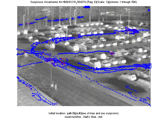
Figure 1: Suspiciousness analysis of paths in an infrared image sequence.
Table 2: Average precision, recall, and F-score in experiments.
|
|
Color Sequences |
Infrared Sequences |
|||||
|
Precision |
Recall |
F-score |
Precision |
Recall |
F-score |
||
|
All |
Suspicious objects (11) |
.45 |
.70 |
.55 |
.71 |
.80 |
.75 |
|
Loitering (16) |
.69 |
.74 |
.71 |
.89 |
.79 |
.84 |
|
|
Other behaviors (26) |
.61 |
.67 |
.64 |
.68 |
.63 |
.63 |
|
|
Total |
.60 |
.69 |
.64 |
.61 |
.72 |
.66 |
|
|
Accel. factor |
Suspicious objects (11) |
.52 |
.83 |
.64 |
.47 |
.87 |
.61 |
|
Loitering (16) |
.67 |
.57 |
.62 |
.61 |
.62 |
.62 |
|
|
Other behaviors (26) |
.53 |
.50 |
.51 |
.67 |
.46 |
.55 |
|
|
Total |
.57 |
.61 |
.59 |
.59 |
.62 |
.60 |
|
Results show only about third of the flagged behavior would be false alarms, and only about one third of the true suspicious behavior would be missed.� Performance could also be improved with better segmentation, since most of the errors were due to it, but that will not be an issue when data comes from sensor networks.� Infrared imagery was more successful than color imagery, thanks to its better segmentation of people.
The acceleration norm factors significantly outperformed the other factors.� In fact, all but 9% of the overall performance can be attributed to it.� This confirms our hypothesis that, at least for the kinds of behaviors depicted in this video, gross body motion is sufficient to indicate most suspicious activities.
4. Automated analysis of groups of people
Many suspicious activities occur in groups of people.� People are often found together, and how they are interacting can be a valuable clue in analyzing their purposes.� We seek general-purpose metrics that can characterize a wide range of settings, and we seek methods that are easy to automate.� We have been analyzing images from training exercises at the Marine base at Twenty Nine Palms in California (U.S. Marine Corps, 2005).� We are installing a network of cameras to do tracking using the approach of (Aguilar-Ponce, 2007).� While this work uses images, it could also use data obtained from sensors such as meter-resolution GPS units.
We assume a two-dimensional world where we have a complete
terrain model.� We assume we have knowledge for each of N persons of just their
position and their orientation, so each is a triple ![]() .�
If necessary,
.�
If necessary, ![]() �values can be estimated
from the direction in which people are heading, though preferably it should
obtain and use head orientation.� We have a Matlab program that obtains these
for a given picture by having a user click on pairs of locations in a picture
to indicate first person positions and directions they are facing (by clicking
on a second point indicating the direction), locations of bottoms of walls, and
locations of bottoms of doors and windows (though other researchers on our ONR
project will eventually automate the extraction of this data from video).� A
perspective transformation is converts image coordinates to real-world
coordinates.� Figure 2 shows an example of the input to our program to compute
such metrics, and Figure 3 shows the inferred terrain for Figure 2.
�values can be estimated
from the direction in which people are heading, though preferably it should
obtain and use head orientation.� We have a Matlab program that obtains these
for a given picture by having a user click on pairs of locations in a picture
to indicate first person positions and directions they are facing (by clicking
on a second point indicating the direction), locations of bottoms of walls, and
locations of bottoms of doors and windows (though other researchers on our ONR
project will eventually automate the extraction of this data from video).� A
perspective transformation is converts image coordinates to real-world
coordinates.� Figure 2 shows an example of the input to our program to compute
such metrics, and Figure 3 shows the inferred terrain for Figure 2.

Figure 2: Image 40.
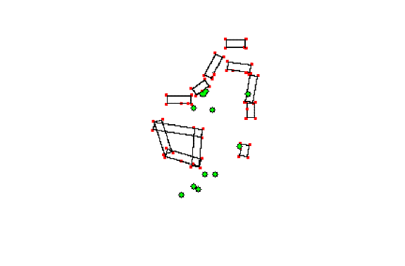
Figure 3: Terrain inferred for Figure 2 viewed from above.
4.1. Static analysis of positions
One class of metrics can be computed at a single instant of time.� Mostly we seek scale-free metrics that refer to the form of the pattern of people.
Dispersion
Dispersion is the degree to which people are spread out across the terrain.� One metric is to measure the average distance between persons.� However, this formula gives equal weight to all pairs of persons.� It is really only the distance to the nearest person or nearest few persons that matters for each person, as is suggested by work on automated robot dispersion for coordinated tasks (Mataric, 1994; Hsu, Jian, & Lian, 2006).� Thus we could use:

The outer summation computes the mean distance over all
persons.� A problem with this metric is that its units are distances, and we
prefer metrics that range between 0 and 1 to indicate unsuitability of an array
of persons.� Assume there is some optimum distance ![]() �between
two persons, a distance that permits communication yet separates them enough to
provide sufficient dispersion for safety.� We can use sigmoid functions to map
distances to the range 0 to 1, plus a logarithm since the ratio of sizes
matters rather than the absolute difference in sizes:
�between
two persons, a distance that permits communication yet separates them enough to
provide sufficient dispersion for safety.� We can use sigmoid functions to map
distances to the range 0 to 1, plus a logarithm since the ratio of sizes
matters rather than the absolute difference in sizes:
![]()
Alternatively, we could use the unevenness of the distribution of persons as a metric, since unevenly distributed persons suggest dispersion problems.� This would be:

This is 0 when the persons are evenly distributed.� To normalize and keep the value of the metric between 0 and 1, we should use:
![]()
Linearity
Another kind of dispersion is along a line of sight since people in columns are more likely to be military or paramilitary.� So besides the above forms of dispersion, we should check the relative collinearity of the group.� We can use the square of the value of the Pearson correlation coefficient:

Another useful linearity metric N1 is the number of distinct lines formed by the persons within a certain maximum amount of deviation.�� For this it is more appropriate to give a recursive algorithm rather than a formula:
function countcolumns(S)
Let S be the set of persons.
If the size of S is 0 or 1, return 0.
If the size of S is 2, return 1.
Else for each pair of persons, count the number of other persons lying within a threshold distance of the line formed by the pair.
Choose the pair with the largest such count, and eliminate these from the set.
Recurse on the set of the remaining persons; return one plus the column count on the remaining persons.
A related metric N2 could be the number of clusters of persons within a threshold.� Low values of this could be appropriate at base, but not generally elsewhere.� We can use the minimum spanning tree algorithm to find this.
Both N1 and N2 depend on their thresholds.� Since we can see interesting phenomena at different values of these thresholds, it is helpful to compute the metric for a range of thresholds.� A systematic way is to plot the number of clusters as a function of the threshold; stretches of this graph that are flat for a significant distance represent important latent structure in the data.� For instance, Figures 4 and 5 show graphs for N1 and N2 as a function of threshold persons for the picture in Figure 2.� Figure 4 shows that three linear clusters is a good way to describe the data, and Figure 5 shows that four positional clusters is a good way to describe the data (in Figure 2, the people in the left foreground, the people at the left back, and the two guard persons stationed on the right).
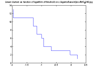
Figure 4: Number of linear clusters (N1) as function of threshold logarithm for persons in Figure 2.

Figure 5: Number of positional clusters (N2) as function of threshold log for persons in Figure 2.
Immobility
Another key safety factor is the degree to which persons can "escape" a potential unsafe situation such as adversarial fire.� This would be low among closely spaced buildings and in cul-de-sacs.� We can measure this as the ratio of the area that can be reached in a given time versus the area that can be reached in the same amount of time on unobstructed terrain; the lower this ratio, the less mobility the persons have.� To find the average area we can do an equicost wavefront propagation about the starting point of the location of the person on a square grid overlain on the terrain.� We assume the wavefront cannot penetrate obstacles inferred from the walls except at doors and windows.� We also assume that other persons form cylindrical obstacles of a radius of three feet for the wavefront, since it is impolite to come closer than at least that distance to people without their permission.
Both the mean lack of mobility for a person (M1) and maximum lack of mobility (M2) are useful metrics.� To formalize this, let D be the sum of the height and width of the square grid used to model the terrain, w(x,y,j) the number of non-obstacle cells reachable at less than or equal to j steps in the wavefront propagation from (x,y), and f the fraction of non-obstacle cells in the grid.� Then we want:

Figure 6 shows the mobility analysis for the person in the lower left corner of Figure 2.� The darkness of the terrain indicates the estimated time to reach there, based on wavefront propagation.
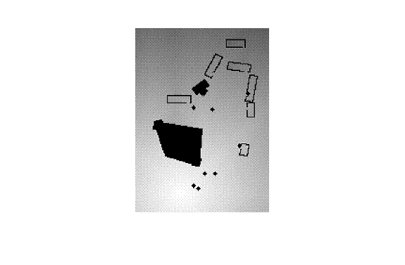
Figure 6: Mobility analysis for the person in the lower left corner of Figure 2.
4.2. Static metrics on visibility
View coverage
A key aspect of situational awareness is ability to see threats.� One way to estimate viewability or visibility of a person is to calculate the fraction of nearby terrain that the person can see.� If we have an image of the persons, we can limit this to terrain visible in the image and within a threshold distance, weighting terrain in importance by the inverse of its distance from the persons (since angular resolution decreases with the inverse distance).� Ability to see terrain should decrease with roughly the cosine of the angle between the terrain and the person's direction of view (Antsis, 1998).� Also, we are primarily concerned with the probability that one person sees a location, and additional persons seeing it does not help much; we will assume that observations of persons are independent.� Some places in the terrain are much more important to see that others because they provide concealment for an adversary: doors, windows, and corners of buildings.� Thus we should give them an extra weighting when assessing average visibility.
This suggests, where ![]() is
the "door constant" that represents the relative importance of the
location (r,c) based on whether it has a door, window, or building corner
there, v(r1,c1,r2,c2) is 1 provided location (r1,c1) is visible from location
(r2,c2) else 0, b is the bearing angle from one location to another, and d is
the distance between locations:
is
the "door constant" that represents the relative importance of the
location (r,c) based on whether it has a door, window, or building corner
there, v(r1,c1,r2,c2) is 1 provided location (r1,c1) is visible from location
(r2,c2) else 0, b is the bearing angle from one location to another, and d is
the distance between locations:
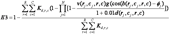
Figure 7 shows the inferred visibilities (the numerator after the summation signs in the above formula) for the terrain in Figure 2.� Here K was 10 for windows, doors, and corners, and 1 otherwise; corners were defined as the free cells diagonally away from a wall end.� Here we pretended the burned-out building in the left foreground was still intact and had occluding walls around it.
Concealment
Another important metric is the degree to which the persons can be seen, as it is often desirable to be concealed as much as possible.� We can use the approach of E3 and compute the average weighted fraction of cells that can see each person.� This time the direction of orientation of the viewer does not matter since we assume they are watching for an adversary, and the scope of the summations is different.

Again, these metrics assume equal visibility at equal distances, and we will need eventually to incorporate the analysis of (Darken and Jones, 2007).
Results with static metrics
We wrote a Matlab program to compute the metrics.�� Walls
are assumed to be infinitely high and doors and windows are assumed to enable
180 degrees of view.� As a demonstration, we evaluate three additional pictures
besides the previous one (image 40), shown below (78, 62, and 81).� Judging by
the results on these (Table 2), metrics D3, U3, P4, N1a, E3, and V4 seem the
best indicators of the differences between human behaviors.
Figure7: Inferred visibilities for the set of soldiers in Figure 2.
Table 3: Metric values on example images from Twenty Nine Palms.
|
Measure / Image number |
40 |
78 |
62 |
81 |
|
K1,number of people |
13 |
6 |
14 |
14 |
|
D2, average distance to closest person for each person |
15.4 |
42.5 |
8.6 |
4.5 |
|
D3, probability the distance is abnormal |
.044 |
.283 |
.328 |
.609 |
|
U2, uniformity of the average distance between persons |
13.6 |
10.6 |
6.4 |
3.37 |
|
U3, probability the uniformity is inadequate |
.756 |
.198 |
.689 |
.696 |
|
P4, square of Pearson correlation coefficient measuring linearity |
.085 |
.613 |
.002 |
.161 |
|
N1a, number of columns using 5 foot grouping threshold |
5 |
2 |
3 |
6 |
|
N2a, number of clusters of persons using 10 foot threshold |
10 |
6 |
7 |
2 |
|
N4, number of apparent conversations |
3 |
0 |
4 |
13 |
|
M1, average lack of mobility of a person |
.08 |
.00 |
.05 |
.24 |
|
M2, maximum lack of mobility of a person |
.10 |
.00 |
.13 |
.76 |
|
E3, average lack of visibility of terrain cells in image area |
.562 |
.284 |
.620 |
.851 |
|
V4, average lack of concealment in image area |
.260 |
.871 |
.158 |
.210 |
|
V5, maximum lack of concealment in image area |
.397 |
.933 |
.300 |
.739 |

Figure 8: Image 78.

Figure 9: Image 62.

Figure 10: Image 81.
4.3. Dynamic metrics
We can also compute metrics over a series of images of persons to assess how they move.� If we know the time between images, we can compute the amount by which the persons move between images.� This requires at least two images.� Easiest is to compute is the speed of the center of gravity of the persons:

Here ![]() �is the number
of persons in image j,
�is the number
of persons in image j,![]() �is the two-dimensional
position of person i in image j, and
�is the two-dimensional
position of person i in image j, and ![]() �is the time of
image j. �Alternatively, we may want to know how evenly the persons move.� This
requires at least three images.� One metric is the norm of the acceleration
vector normalized by the speed, using the positions of the persons:
�is the time of
image j. �Alternatively, we may want to know how evenly the persons move.� This
requires at least three images.� One metric is the norm of the acceleration
vector normalized by the speed, using the positions of the persons:

4.4. Mapping the metrics to the behaviors
The metrics give clues to what people are doing.� Table 3 shows some basic groups behaviors that the metrics will help identify.
Table 4: Expected values of the metrics for five example small-unit behaviors.
|
Behavior |
Random |
Group travel |
Loitering |
Emplacing |
|
K1, number of people |
medium |
medium |
medium |
low |
|
D3, probability the distance between people is large |
medium |
low |
medium |
high |
|
U3, probability the uniformity is low |
high |
medium |
high |
medium |
|
P4, square of Pearson correlation coefficient �measuring linearity |
low |
medium |
low |
low |
|
N1a, number of columns using 5 foot grouping threshold |
high |
medium |
high |
medium |
|
N2a, number of clusters of persons using 10 foot threshold |
medium |
low |
high |
high |
|
N4, number of apparent conversations |
low |
medium |
low |
low |
|
M1, average lack of mobility |
medium |
medium |
low |
low |
|
M2, maximum lack of mobility |
medium |
medium |
low |
low |
|
E3, average lack of visibility |
medium |
medium |
low |
low |
|
V4, average lack of concealment |
high |
high |
medium |
low |
|
V5, maximum lack of concealment |
high |
high |
medium |
low |
5. Acknowledgments
This work was supported in part by the National Research Council under their Research Associateship Program at the Army Research Laboratory, in part by the National Science Foundation under the EXP Program, and in part by the BASE-IT Project sponsored by the Office of Naval Research.� Views expressed are those of the author and do not represent policy of the U.S. Navy.� We are grateful for help from Alex Chan, Jonathan Roberts, E. John Custy, Matthew Thielke, Vishav Saini, Bryant Lee, and Jamie Lin.�
6. References
R. Aguilar-Ponce, A. Kumar, J. Tecpanecatl-Xihuitl, and M. Bayoumi, A network of sensors-based framework for automated visual surveillance, Journal of Network and Computer Applications, Vol. 30, No. 3, pp. 1244-1277, August 2007.
Anstis, S.� Picturing peripheral acuity.� Perception, 27 (1998), pp. 817-825.
Darken, C., and Jones, B., Computer-based target detection for synthetic persons.� Proceedings of BRIMS Spring Simulation Conference, Norfolk, VA, 2007.
Figueiras, J., Schwefel, H.-P., and Kovacs, I., Accuracy and timing aspects of location information based on signal-strength measurements in Bluetooth. �16th IEEE Intl. Symp. on Personal, Indoor, and Mobile Radio Communications, September 2005, pp. 2685-2690.
D. Gibbins, G. Newsam, and M. Brooks, Detecting suspicious background changes in video surveillance of busy scenes, Proc. 3rd IEEE Workshop on Applications of Computer Vision, December 1996, pp. 22-26.
S. Hackwood and P. Potter, Signal and image processing for crime control and crime prevention, in Proc. Intl. Conf. on Image Processing, Kobe, Japan, October 1999, vol. 3, pp. 513-517.
Hsu, W.-H., Jian, Y.-L., & Lian, F.-L.� Multi-robot movement design using the number of communications links.� Proc. Intl. Conf. on Systems, Man, and Cybernetics, Taipei, Taiwan, pp. 4465-4470, October 2006.
Kaplan, E., Leva, J., Milbert, D., and Pavloff, M., Fundamentals of satellite navigation.� In Kaplan, E., and Hegarty, C. (eds.), Understanding GPS: Principles and Applications, Norwood, MA: Artech, 2006, pp. 21-65.
Lee, J., Cho, K., Lee, S., Kwon, T., and Choi, Y., Distributed and energy-efficient target localization and tracking in wireless sensor networks. �Computer Communications, 29 (2006), pp. 2494-2505.
Mataric, M.� Interaction and intelligent behavior.� Technical Report AITR-1495, Artificial Intelligence Laboratory, Massachusetts Institute of Technology, 1994.
T. Meservy, M. Jensen, J. Kruse, D. Twitchell, J. Burgoon, D. Metaxas, and J. Nunamaker, Deception detection through automatic, unobtrusive analysis of nonverbal behavior, IEEE Intelligent Systems, vol. 20, no. 5, pp. 36-43, 2005.
A. Panangadan, M. Mataric, and G. Sukhatme, Detecting anomalous human interactions using laser range-finders.� In Proc. Intl. Conf. On Intelligent Robots and Systems, September 2004, vol. 3, pp. 2136-2141.
G. Powell, L. Tyska, and L. Fennelly, Casino surveillance and security: 150 things you should know.� New York: Asis International, 2003.
N. C. Rowe, Detecting suspicious behavior from positional information.� Workshop on Modeling Others from Observations, Intl. Joint Conference on Artificial Intelligence, Edinburgh, UK, July 2005 (available at www.isi.edu/~pynadath/MOO-2005/7.pdf).
J. Sundram, P. P. Sim, N. C. Rowe, and G. Singh, Assessment of electromagnetic and passive diffuse infrared sensors in detection of suspicious behavior.� International Command and Control Research and Technology Symposium, Bellevue, WA, June 2008.
U.S. Marine Corps, Infantry training and readiness manual.� Directive NAVMC DIR 3500.87, September 2005.
M. Valera and S. Velastin, Intelligent distributed surveillance systems: a review, IEE Proceedings � Vision, Image, and Signal Processing, vol. 152, pp. 192-204, 2005.
D. Wood, In defense of indefensible space, in Environmental Crimonology, P. Brantingham & P. Brantingham, Eds.� Beverly Hills, CA: Sage, 1981, pp. 77-95.
V. Zarimpas, B. Honary, D. Lundt, C. Tanriovert, and N. Thanopoulos, Location determination and tracking using radio beacons. �6th Intl. Conf. on the Third Generation and Beyond, November 2005, pp. 1-5.