NAVAL

POSTGRADUATE

SCHOOL

 

MONTEREY, CALIFORNIA

 

 

 

THESIS

 

Approved for public release; distribution is unlimitedApproved for public release;distribution is unlimited

THIS PAGE INTENTIONALLY LEFT BLANK

REPORT DOCUMENTATION PAGE					Form Approved OMB No. 0704-0188
Public reporting burden for this collection of information is estimated to average 1 hour per response, including the time for reviewing instruction, searching existing data sources, gathering and maintaining the data needed, and completing and reviewing the collection of information. Send comments regarding this burden estimate or any other aspect of this collection of information, including suggestions for reducing this burden, to Washington headquarters Services, Directorate for Information Operations and Reports, 1215 Jefferson Davis Highway, Suite 1204, Arlington, VA 22202-4302, and to the Office of Management and Budget, Paperwork Reduction Project (0704-0188) Washington DC 20503.
1. AGENCY USE ONLY (Leave blank)		2. REPORT DATE  September 2015	3. REPORT TYPE AND DATES COVERED Master�s thesis
4. TITLE AND SUBTITLE  STUDYING URBAN MOBILITY THROUGH MODELING DEMAND IN A BIKE SHARING SYSTEM					5. FUNDING NUMBERS
6. AUTHOR(S)  Kang, Shian Chin
7. PERFORMING ORGANIZATION NAME(S) AND ADDRESS(ES) Naval Postgraduate School Monterey, CA  93943-5000					8. PERFORMING ORGANIZATION REPORT NUMBER
9. SPONSORING /MONITORING AGENCY NAME(S) AND ADDRESS(ES) N/A					10. SPONSORING / MONITORING  AGENCY REPORT NUMBER
11. SUPPLEMENTARY NOTES  The views expressed in this thesis are those of the author and do not reflect the official policy or position of the Department of Defense or the U.S. Government.  IRB Protocol number ____N/A____.
12a. DISTRIBUTION / AVAILABILITY STATEMENT  Approved for public release; distribution is unlimitedApproved for public release;distribution is unlimited					12b. DISTRIBUTION CODE
13. ABSTRACT (maximum 200 words)    Resource allocation problems occur in many applications.  One example is bike-sharing systems, which encourage the use of public transport by making it easy to rent and return bicycles for short transits.  With large numbers of distributed kiosks recording the time and location of rental transactions, the system acts like a sensor network for movement of people throughout the city.  In this thesis, we studied a range of machine-learning algorithms to predict demand (ridership) in a bike-sharing system, as part of an online competition.  Predictions based on the Random Forest and Gradient Boosting algorithms produced results that ranked amongst the top 15% of more than 3000 team submissions.  We showed that the mandated use of logarithmic error as the evaluation metric overemphasizes errors made during off-peak hours.  We systematically experimented with model refinements and feature engineering to improve predictions, with mixed results.  Reduction in cross-validation errors did not always lead to reduction in test-set error.  This could be due to overfitting and the fact that the competition test set was not a random sample.  The approach in this thesis could be generalized to predict use of other types of shared resources.
14. SUBJECT TERMS Machine-Learning, Bike-Sharing, Demand Forecasting						15. NUMBER OF PAGES 41
						16. PRICE CODE
17. SECURITY CLASSIFICATION OF REPORT Unclassified	18. SECURITY CLASSIFICATION OF THIS PAGE Unclassified			19. SECURITY CLASSIFICATION OF ABSTRACT Unclassified		20. LIMITATION OF ABSTRACT   UU

NSN 7540-01-280-5500                                                                                                              Standard Form 298 (Rev. 2-89)

                                                                                                                                                    Prescribed by ANSI Std. 239-18

THIS PAGE INTENTIONALLY LEFT BLANK

 

 

Approved for public release; distribution is unlimitedApproved for public release;distribution is unlimited

 

 

STUDYING URBAN MOBILITY THROUGH MODELING DEMAND IN A BIKE SHARING SYSTEM

 

 

Shian Chin Kang

Civilian, Defence Science and Technology Agency, Singapore

Dipl�me d'Ing�nieur, ESTP, 2005 

M.Sc., NUS, 2009

 

 

Submitted in partial fulfillment of the

requirements for the degree of

 

 

MASTER OF SCIENCE IN COMPUTER SCIENCE

 

from the

 

NAVAL POSTGRADUATE SCHOOL

September 2015

 

 

 

 

 

Approved by:              Neil C. Rowe

Thesis Advisor

 

 

 

Thomas W. Otani

Co-Advisor

 

 

 

Peter Denning

Chair, Department of Computer Science

THIS PAGE INTENTIONALLY LEFT BLANK

 

ABSTRACT

Resource allocation problems occur in many applications.  One example is bike-sharing systems, which encourage the use of public transport by making it easy to rent and return bicycles for short transits.  With large numbers of distributed kiosks recording the time and location of rental transactions, the system acts like a sensor network for movement of people throughout the city.  In this thesis, we studied a range of machine-learning algorithms to predict demand (ridership) in a bike-sharing system, as part of an online competition.  Predictions based on the Random Forest and Gradient Boosting algorithms produced results that ranked amongst the top 15% of more than 3000 team submissions.  We showed that the mandated use of logarithmic error as the evaluation metric overemphasizes errors made during off-peak hours.  We systematically experimented with model refinements and feature engineering to improve predictions, with mixed results.  Reduction in cross-validation errors did not always lead to reduction in test-set error.  This could be due to overfitting and the fact that the competition test set was not a random sample.  The approach in this thesis could be generalized to predict use of other types of shared resources. 

THIS PAGE INTENTIONALLY LEFT BLANK

TABLE OF CONTENTS

I.             INTRODUCTION.................................................................................. 1

A.           STUDYING URBAN MOBILITY ThROUGH BIKE SHARING SYSTEMS................................................................ 1

B.           The Bicycle-Sharing Problem and Competition......................................................................... 1

C.           Competition RULES........................................................... 2

D.           Approach................................................................................ 4

E.           Contributions.................................................................... 4

F.           Overview of Thesis.......................................................... 4

G.          TERMINOLOGY....................................................................... 5

II.           USING MACHINE LEARNING ALGORITHMS FOR DEMAND FORECASTING..................................................................................... 6

A.           RIDGE REGRESSION.............................................................. 7

B.           GRADIENT Boosting.......................................................... 7

C.           Support Vector Regression...................................... 8

D.           Random Forest................................................................... 8

III.         MODELING APPROACH.................................................................. 10

A.           DETAILS OF THE DATASET.............................................. 10

B.           EVALUATION CRITERIA.................................................... 12

C.           DATA PRE-PROCESSING.................................................... 12

D.           Modeling Approach...................................................... 13

1.            First-cut screening for best algorithm.......................... 13

2.            Fine-tuning the Model................................................... 14

a.            Building two separate models for casual users and registered users.................................................... 14

b.            Feature selection................................................. 14

c.            Introducing Features to Improve Prediction for Wee Hours........................................................... 15

d.            Introducing Features to Account for Temporal Dependencies...................................................... 15

3.            Final model..................................................................... 16

IV.         Results.............................................................................................. 17

A.           ACCOUNTING FOR MISSING DATA................................ 17

B.           ANALYSIS OF DATA............................................................. 17

C.           Algorithm Selection from first-pass modeling.............................................................................. 22

D.           Variable Importance FROM RANDOM FOREST 23

E.           DISCUSSION ON THE RMSLE EVALUATION FUNCTION............................................................................... 25

F.           MODEL FINE-TUNING USING THE RANDOM FOREST ALGORITHM........................................................................... 27

1.            Predicting Casual and Registered demand separately.......................................................................................... 28

2.            Feature selection............................................................ 28

3.            Adding Features to Improve Prediction for Wee Hours......................................................................................... 31

4.            Accounting for Trends (Moving Average and Week Number)......................................................................... 31

5.            Combining the New Features....................................... 32

V.           Chapter 6: Conclusion............................................................ 34

A.           SUMMARY OF FINDINGS.................................................... 34

B.           LESSONS LEARNED............................................................. 35

C.           RELATED WORK................................................................... 36

List of References................................................................................ 38

initial distribution list.................................................................... 41

 

 

THIS PAGE INTENTIONALLY LEFT BLANK

LIST OF FIGURES

Figure 1.             Growth in Hourly Demand (7am to 7pm) from 2011 to 2012.... 19

Figure 2.             Seasonal Variations..................................................................... 19

Figure 3.             Hourly Demand for Casual, Registered and All Users on Working Days vs. Non-Working Days....................................................... 20

Figure 4.             Decision Tree for Registered Users (7 am to 7 pm).................... 21

Figure 5.             Decision Tree for Casual Users (Depth = 4)................................ 22

Figure 6.             Sub-Tree for Casual Users from Rightmost Node in Figure 5.... 23

Figure 7.             Logarithmic Error vs. Actual Count............................................ 27

Figure 8.             Error in Logarithmic Demand vs Actual Count (Decision Tree). 28

 

THIS PAGE INTENTIONALLY LEFT BLANK

LIST OF TABLES

Table 1.               Detailed Description of Dataset (Independent Variables).......... 11

Table 2.               Detailed Description of Dataset (Dependent Variables)............. 11

Table 3.               Independent Variables after Data Pre-Processing....................... 12

Table 4.               Dependent Variables after Data Pre-Processing......................... 13

Table 5.               List of R Packages Used............................................................. 14

Table 6.               Features to Improve Prediction for Off-Hours........................... 15

Table 7.               Features to Account for Temporal Dependencies....................... 16

Table 8.               RMSLE and Ranking obtained by 5 different algorithms.......... 23

Table 9.               Variable Importance for Registered Users.................................. 24

Table 10.            Variable Importance for Casual Users......................................... 24

Table 11.            Missed Predictions vs. Logarithmic Error................................... 25

Table 12.            Effect of using separate models to predict registered and casual users vs. using a single model to predict count........................... 28

Table 13.            Variable-Selection Scheme.......................................................... 29

Table 14.            Results of Cross Validation......................................................... 30

Table 15.            Variables that Produced our Best Test-Set RMSLE................... 30

Table 16.            Adding Features to Improve Predictions during Wee Hours...... 31

Table 17.            Adding Features to Account for Trends (Moving Average and Week Number)............................................................................ 32

Table 18.            Combining New Features with Base Model............................... 32

 

 

THIS PAGE INTENTIONALLY LEFT BLANK

LIST OF ACRONYMS AND ABBREVIATIONS

 

ARIMA                      Autoregressive Integrated Moving Average

RMSLE                       Root-Mean-Squared Logarithmic Error

SVM                           Support Vector Machine

 

 

 

THIS PAGE INTENTIONALLY LEFT BLANK

 

THIS PAGE INTENTIONALLY LEFT BLANK

 

 ACKNOWLEDGMENTS

I am truly grateful for the guidance and kind support of my advisors, Prof. Neil Rowe and Prof. Thomas Otani.  I would like to thank Prof. Lyn Whitaker for her instruction and for keeping classes interesting and stimulating.  I am thankful to DSTA, particularly Mr. Pang Chung Khiang, without whom none of this would have been possible.  Last but not least, I would like to thank my wife, Fei San, and my son, Jin Yi, for your wonderful companionship, and for allowing me to complete this thesis with ease of mind despite the challenges we have had to face.

 

THIS PAGE INTENTIONALLY LEFT BLANK

 

I.                  INTRODUCTION

 

A.                STUDYING URBAN MOBILITY ThROUGH BIKE SHARING SYSTEMS

Population growth and rapid urbanization create increasing demand for public services such as public transportation, causing considerable strain to the infrastructure of cities around the world (Belissent, 2010).  Numerous �smart city� initiatives have been launched to leverage information and communications technology to meet these demands with limited resources.  A recurring challenge is how one can derive insights or actionable intelligence from the increasing amounts of data being collected.  In this thesis, we tackle an instance of this problem by studying urban mobility through data collected from a bicycle-sharing system.  We will use machine-learning algorithms to predict the demand for bicycles based on historical rental patterns and weather information.  This is a different approach to traditional time-series analysis used in marketing theory (see Chapter II).

B.                 The Bicycle-Sharing Problem and Competition

Bike-sharing systems allow urban commuters to rent bicycles from automated kiosks at one location and to return them at another location.  Rental prices are often designed to encourage short trips lasting less than an hour.  One of the key ideas behind bicycle sharing systems is to provide a �last mile� solution for commuters to travel between a transit point (e.g. subway station) and their home or workplace, thereby reducing their reliance on vehicles.  Bike-sharing systems have existed since the 1960s but only seen widespread adoption in the past decade thanks to advances in information technology (Shaheen, Martin, Chan, Cohen, and Pogodzinski, 2014).  As of June 2014, there were public bike-sharing systems in 712 cities globally, collectively operating around 37,500 stations and 806,200 bicycles (Shaheen et al., 2014).  Due to the extensive use of technology to automatically track rentals and returns, bike-sharing systems generate much data on trips.  From this perspective, bike-sharing systems are analogous to a sensor network and the data generated presents an opportunity for transport planners and researchers to better understand and support urban mobility by mining the dataset (Kaggle Inc., 2014).

In this thesis, we use a range of machine-learning techniques to model and predict the hourly demand for bicycles in a bike-sharing system by mining data on historical rental patterns and weather information.  This problem was posted as a contest on the online data-mining competition platform Kaggle (www.kaggle.com). The dataset was provided by Fanaee-T and Gama (2013) and was hosted in the University of California, Irvine (UCI) machine-learning repository.  The bike-sharing system in question was Capital Bikeshare which operated 1650 bicycles and 175 stations across the District of Columbia, Arlington County, and the City of Alexandria in Nov 2012 (LDA Consulting, 2013).  The dataset contained the aggregate hourly demand for bikes and weather information such as temperature, humidity and wind speed (see Chapter III for details on the dataset).  Public holidays were also indicated in the dataset. 

The online competition was held between 28 May 2014 and 29 May 2015.  Although the official competition is now closed, Kaggle members are still able to make unofficial submissions for learning purposes, as with all other Kaggle-hosted competitions.

C.                Competition RULES

The training set for the competition included the hourly demand for bicycles (i.e. number of bicycles currently rented out) and weather conditions in the first 19 days of each month in 2011 and 2012.  The test set is made up of the remaining 9�12 days of each month.  Participants were not allowed to use any other data sets other than one provided (for instance, they could not use weather data from other sources).  The competition rules state that the hourly demand for the test set must be predicted �using only information available prior to the rental period� (Kaggle Inc., 2014).   This rule caused some controversy on online forums linked to the competition.  While the rule was imposed to introduce more realism, it creates challenges from a modeling perspective.  Instead of building a single model based on the entire training set, 24 sub-models must be built using progressively more data as each month progresses.  It means that predictions for the earlier months are based on less data.  For example, the predictions for 20th Jan 2011 to 31st Jan 2011 can only be made based on 19 days of data between 1 Jan 2011 and 19 Jan 2011.

Judging from the online forums linked to the competition and code that was published by some participants (publishing code did not go against the rules as long as the code was shared openly to everyone), we noticed many teams did not follow the abovementioned rule.  Although this cannot be easily verified, most teams that were ranked highly appear to have used the entire dataset to build a single model to predict demand for all the rental periods in the test set.  Predictions using 24 sub-models were essentially extrapolations while predictions made by the single model, apart from being trained on a much larger dataset, were interpolations and can be expected to be more accurate.  Despite the controversy, the competition rules remained unchanged throughout the period of the competition and it was not clear how the organizers could tell if a submission followed the rules, since only the results needed to be submitted.  Fortunately, the competition was for �fun and practice� (Kaggle Inc., 2014), so it did not involve a prize or other benefits.  Since the competition allowed for teams to submit two result sets, we made one submission that followed the rules (using 24 sub-models) and one which did not (using a single model).  We added comments in the submission which clearly flagged out which submission did not follow the rules.  Our single model submission ranked 141st out of 3252 teams, and our 24 sub-model submission would have us rank 755th.  Since the full dataset was relatively small for a data-mining application (19 days x 24 months = 456 days of data), we decided it was not meaningful to use subsets of the data for training.  To study the problem meaningfully, the rest of this thesis will be based on a single-model approach. 

Taking part in the competition provided more excitement for our work and an online community that is actively engaged in the same problem.  Many participants have posted their solutions online.  From reading some of the solutions, we note that many teams have taken similar approaches to the problem and have had similar findings.  In this thesis, we can neither claim to have a completely novel approach nor the best solution, since 140 teams have a better score than us on the test set.  Nonetheless, we hope to add value to the discussion by sharing findings from the experiments we carried out, including those that worked and those that did not.

D.                Approach

In the first stage, we tested a range of machine-learning algorithms to identify those that worked best for the problem.  The algorithms we tested were Ridge Regression, Support Vector Regression, Gradient Boosting, and Random Forest.  We used a range of software packages in R, a popular programming language for data analysis, tweaking the parameters extensively to try to maximize each algorithm�s performance for the training and test set.  After identifying the most suitable algorithm, we tried to improve the model further by fine-tuning the modeling in a second stage, for example by predicting demand from casual users and registered users separately.  This two-stage approach was adopted to reduce the dimensionality of the problem.

E.                 Contributions

Through this thesis, we provide empirical results of applying a range of machine-learning algorithms to predict demand for a service.  We found that Random Forest and Gradient Boosting produced the best results for this application.  From analyzing the results and a simple scenario analysis, we showed that using RMSLE as the evaluation metric overemphasizes missed predictions during off-peak hours.  We systematically fine-tuned the Random Forest model through a series of experiments.  We showed that reductions in cross-validation error did not necessarily result in improvements in the test-set error.  The lessons learned from this study could be applied to similar problems to predict demand for other forms of transport, goods, or logistic services, and may be of particular interest to marketing, operations, and infrastructure planners.

F.                 Overview of Thesis

In Chapter II, we provide a brief review of the regression algorithms used in this thesis.  In Chapter III, we discuss the variables in the dataset, the evaluation function as well as our modeling approach, including data preprocessing and the modeling refinements.  In Chapter IV, we present the results of our findings.  Finally, in Chapter V, we provide a summary of lessons learned and possible follow on work.

G.                TERMINOLOGY

The field of machine learning is influenced by other fields such as statistics (data mining) and computer science (artificial intelligence).  This is reflected in the different terms used to describe the same concept or object.  In this thesis, we use some terms interchangeably depending on what is most commonly used in academic literature.  �Target variable� and �dependent variable� refer to the variable to be predicted by the model (i.e. hourly demand).  �Input variables�, �independent variables�, �features�, or �factors� refer to variables that are used as input to the model.  They are also referred to as �attributes� in some literature.  �Model� refers to a theory relating the independent variables to the output variable, and is the end product of running one or more machine-learning algorithm on a training set.  A model can make predictions when it is given input variables from a test set.  A modeling approach refers to how we model a problem, which translates to how we pre-process data, how we select features, and how we chain multiple algorithms and sub-models together.

II.               USING MACHINE LEARNING ALGORITHMS FOR DEMAND FORECASTING

Demand forecasting can lead to better resource allocation decisions for any organization concerned with meeting customer expectations, improving operational efficiency, and reducing wastage.  A wide range of methods for demand forecasting are in use, particularly in marketing theory.  They can be categorized into quantitative and non-quantitative methods.  A classical quantitative approach is the use of time-series analysis methods like ARIMA (i.e. autoregressive integrated moving average) where we decompose a time series into long term trends, seasonal and cyclical variations and random fluctuations.  Methods like ARIMA are called autoregressive because the forecast is based solely on past values of the demand itself.  Its advantage is that one can produce models easily by observing the demand over time.  However, autoregressive methods are unable to take into account causal factors that impact demand, simply because they do not take in input other than past values of demand.  For example, an exceptionally warm week in winter may cause bicycle rentals to spike beyond seasonal norms.  An autoregressive model would not be able to predict this spike if it is unable to take temperature as an input.

In this thesis we studied four machine-learning algorithms for predicting hourly demand for bicycles.  First, we applied Ridge Regression, a linear-regression algorithm which serves as a baseline for comparison.  Next, we studied three relatively modern nonlinear learning algorithms, Gradient Boosting, Support Vector Machines, and Random Forest.  The algorithms were selected based on a study by Caruana and Niculescu-Mizil in 2006.  By evaluating 10 supervised learning methods using 11 different test problems across a wide range of performance metrics, Caruana and Niculescu-Mizil (2006) highlighted that �boosting, random forests, bagging, and SVMs achieve excellent performance that would have been difficult to obtain just 15 years ago�.  It should be highlighted that Caruana and Niculescu-Mizil�s research was done on binary classification problems, unlike the regression problem in this thesis, and that the findings of their research were more nuanced than simply saying these were the three best algorithms available. Nonetheless, the selected algorithms performed well in Caruana and Niculescu-Mizil�s research on the mean-squared error metric, which is also what we are using in this thesis as the evaluation function.  We provide a brief review of these four regression algorithms.

A.                RIDGE REGRESSION

Linear regression methods based on ordinary least-squares are easy to implement and interpret.  Simple linear regression works well for simple problems with limited number of independent variables.  However, it can be prone to overfitting when there is a large number of independent variables.  This problem could be solved either by reducing the number of variables (subset selection) or shrinkage methods (Hastie, Tibshirani, and Friedman, 2009).  One well known shrinkage method is Ridge Regression where we introduce a complexity parameter, λ, when minimizing a �penalized residual sum of squares� to shrink the regression coefficients towards zero (Hastie et al., 2009).  This has the effect of penalizing complex models (i.e. models with many non-zero regression coefficients).  Although we do not expect Ridge Regression to do particularly well against non-linear methods, it serves as a baseline for comparison with other methods.  In this thesis we use the R package glmnet for its implementation of Ridge Regression (Friedman, Hastie and Tibshirani, 2010).

B.                 GRADIENT Boosting

Ensemble methods refer to the combination of a set of individually trained classifiers to produce predictions that are better than that produced by any of the constituent classifiers (Opitz and Maclin, 1999).  Boosting is a class of ensemble learning which combines a set of weak learners into a strong learner (Freund and Schapire, 1997).  In 1997, Freund and Schapire introduced Adaboost, or adaptive boosting, which has since become one of the most well-known boosting algorithms.  In Adaboost, each subsequent classifier is trained on a reweighted dataset obtained by increasing the relative weight of instances that are misclassified by preceding classifiers (Hastie et al., 2009).  In this thesis, we use the gbm (Gradient Boosting Machine) package (Ridgeway, 2012) in R that implements Adaboost using Friedman�s gradient descent algorithm.  Gradient Boosting Machines uses decision trees as weak classifiers which it combines. 

C.                Support Vector Regression

The idea for support vector machines (SVM) originated in the 1960s as a linear classification method (Vapnik and Lerner, 1963).  In 1996, a version of SVM called Support Vector Regression was introduced by Vapnik, Golowich, and Smola (1997).  By late 1990s, support vector machines have emerged as one of the leading classifiers for OCR, object recognition, as well as regression (Smola and Sch�lkopf, 2004).  The SVM algorithm is based on finding the hyperplane that best separates two classes in a multi-dimensional space.  In this thesis we use the svm function in the e1071 R package (Dimitriadou, Hornik, Leisch, Meyer, and Weingessel, 2009) to perform Support Vector Regression on the bicycle-sharing dataset.  We tuned the model by varying the basis function, cost parameter C, and gamma (for the radial basis function).

D.                Random Forest

Random Forest (Breiman, 2001) is another ensemble method which is currently very popular.  The algorithm makes use of a collection of de-correlated decision trees to make a more accurate prediction.  Each tree is constructed using a bootstrapped sample of the training set (i.e. a sample that is of same size as the training set, but sampled with replacement).  When growing each tree, at each step, a random subset (of size m) of all the independent variables is chosen as candidates for splitting, and the best split is chosen from these m variables (Hastie et al., 2009).  Due to the randomness of their training set and features, each tree may produce a different prediction for the same instance in the test set.  For classification problems, each tree predicts a class, and the mode of the votes (most common class) is chosen as the result.  For regression problems, each tree predicts a value by taking the mean of the target variable across all instances in the same terminal leaf node.  The mean of the prediction across the trees is then taken and used as the final prediction.  Through the voting mechanism, the random forest method corrects for the tendency of each decision tree to overfit the training set.  According to Hastie et al. (2009), the performance of random forests is very similar to boosting, and they are simpler to train and tune.  In this thesis, we use the randomForest R package (Liaw and Wiener,2012), and mainly tuned the number of trees (ntree) and the number of variables randomly sampled (mtry).

III.           MODELING APPROACH

In this chapter, we provide more details on the variables in the dataset, the evaluation criteria for the competition, and the data pre-processing we performed before applying the four machine-learning algorithms. Finally, we describe the experiments to fine-tune the models and improve prediction accuracy once the best learning algorithm was chosen.

A.                DETAILS OF THE DATASET

Capital Bikeshare is a publicly-owned and privately-operated bike-sharing system.  Members of the public can use the bicycles docked at kiosks distributed around District of Columbia, Arlington County, Alexandria and Montgomery County.  Non-registered users can use their credit cards directly at each station to join as members for 24h ($8) or 3-days ($17).  This gives them to right to make as many trips as they wish during this period.  The first 30 min of each trip is free, before additional fees are charged.  This discourages users from holding onto a bicycle for extended periods.  Regular users can sign up for 30-day ($28) or annual memberships ($85) that offer savings over short-term memberships.

The data for the Kaggle competition was provided by Fanaee-T and Gama (2013), who combined data from Capital Bikeshare (https://www.capitalbikeshare.com/trip-history-data) and weather information from Freemeteo (http://www.freemeteo.com).  The dataset included datetime, season, holiday, workingday, weather, temp, atemp, humidity windspeed, casual, registered and count.  Tables 1 and 2 present the types of independent variables and the dependent variables respectively, including a brief description and possible values each variable can take.  There is an instance of each of these variables for each hour in the first 19 days of each month.  The full description of the dataset, rules of competition, and evaluation criteria are available on the competition webpage (https://www.kaggle.com/c/bike-sharing-demand).

 

                          Table 1.  Detailed Description of Dataset (Independent Variables)

	Independent Variables	Description
1	datetime	hourly date + timestamp (e.g. 1/2/2011  7:00:00 AM)
2	season	1 = spring, 2 = summer, 3 = fall, 4 = winter
3	holiday	1 = holiday, 0 = not holiday
4	workingday	1 = working day, 0 = holiday or weekend
5	weather	1 = Clear, Few clouds, Partly cloudy, Partly cloudy  2 = Mist + Cloudy, Mist + Broken clouds, Mist + Few clouds, Mist 3 = Light Snow, Light Rain + Thunderstorm + Scattered clouds, Light Rain + Scattered clouds  4 = Heavy Rain + Ice Pallets + Thunderstorm + Mist, Snow + Fog
6	temp	temperature (Celsius)
7	atemp	"feels like" temperature (Celsius)
8	humidity	relative humidity (%)
9	windspeed	windspeed (km/h)

                             Table 2.  Detailed Description of Dataset (Dependent Variables)

	Dependent Variables	Description
1	casual	number of non-registered user rentals initiated
2	registered	number of registered user rentals initiated
3	count	number of total rentals (To be predicted)

 

As explained in Chapter 1, the training set contains data for the first 19 days of each month in 2011 and 2012, i.e. Jan 2011 to Dec 2012.  There are three dependent variables, namely casual, registered and count.  Casual refers to the number of rentals made by non-registered users for 1-day to 3 day passes.  Registered refers to the number of rentals made using a monthly or annual pass.  Count is the simply the sum of casual and registered.  The test set contains the 9 independent variables for each hour in the last 9 to 12 days of each month, from which competitors need to predict only the count.  It should be highlighted that count refers to the number of bicycles that are actually checked out.  Strictly speaking, the provided data does not give the actual demand, as that would include users who wanted a bike but did not manage to get one, for example, if the kiosk had run out of bikes.

B.                 EVALUATION CRITERIA

Submissions were to be evaluated using the root-mean-squared logarithmic error (RMSLE), which is calculated as follows (https://www.kaggle.com/c/bike-sharing-demand/details/evaluation):

In the RMSLE equation, n is the number of hours in the test set, and p_i and a_i are the predicted count and the actual count for a given hour respectively.  Taking the logarithmic error ensures that missed predictions for peak hours do not overly dominate those for off-peak hours.  However, as we will discuss later, the RMSLE overcompensates for errors during off-peak hours from an economic perspective.

C.                DATA PRE-PROCESSING

Some data pre-processing was necessary to prepare the data set for the selected machine-learning algorithms.  The single datetime variable was split into 4 separate independent variables: year, month, day (of the week) and hour.  This expanded the set of independent-variable types from 9 to 12 (see Table 3).  Variable 1 to 8 were modeled as categorical variables (or �factors� in R terminology) whereas variables 9 to 12 were modeled as numeric variables.

                                       Table 3.  Independent Variables after Data Pre-Processing

 

Instead of using the actual numbers for the casual, registered and count directly to train the algorithms, we used their logarithm i.e. log(casual+1), log(registered+1) and log(count+1) as the target variables to be predicted (see Table 4).  This was done to mirror the RMSLE used as the evaluation function.

                                          Table 4.  Dependent Variables after Data Pre-Processing

The natural log of the hourly demand was taken to mirror the RMSLE evaluation function used in the competition.

D.                Modeling Approach

1.                  First-cut screening for best algorithm

Even with only four algorithms and a relatively manageable dataset, it was still time-consuming to completely explore the permutations of tuning parameters for each algorithm and the different modeling approaches that were possible.  As a first pass, we used the four algorithms covered in Chapter 2 to predict log count.  In this screening phase, we used the test-set error directly to evaluate the algorithms instead of cross-validation.  For each algorithm, we tuned the parameters diligently using a grid search, but in a non-exhaustive manner.  We experimented with the scikit-learn machine-learning library for Python and a range of R packages before settling on R.  We achieved similar performance on both R and Python, but chose R because we were relatively familiar with the syntax and the RStudio IDE.  Table 5 presents the R packages that were used.

                                                                             Table 5.  List of R Packages Used

 

2.                  Fine-tuning the Model

Once we selected our best algorithm (i.e. Random Forest), we proceeded to experiment with fine-tuning our model to improve prediction accuracy.  By fine-tuning the model, we are referring to modifications other than tweaking the parameters of the learning algorithm, for example, adding or removing features, or building separate sub-models, etc.

a.                  Building two separate models for casual users and registered users

Casual users and registered users are likely to exhibit different behaviors and be affected differently by weather conditions or whether it is a public holiday.  An obvious approach is to train two separate models for casual and registered and summing up their respective predictions.  However, it is not obvious that it would improve the prediction accuracy over learning and predicting the aggregate (count) directly due to possible interaction effects.

b.                  Feature selection

In the algorithm-screening phase, we used all available independent variables as features.  However, our dataset contains multiple correlations and potentially weak features.  For example, working day is clearly correlated with weekday and holiday, and season is correlated with month.  Each of the 4 algorithms tested contains a mechanism to deal with redundant features and overfitting. For example, Ridge Regression uses regularization as described in Chapter 8, and Random Forest randomizes the features that are used to each tree.  Feature selection is another possible approach to improve prediction accuracy by directly reducing the initial number of features used to train the model.  While this can be done programmatically, we do this manually in this thesis.

c.                   Introducing Features to Improve Prediction for Off-Hours

From our analysis of the results and RMSLE metric, we noticed that errors during off-peak hours, particularly between midnight and 6 AM., contributed significantly to the overall RMSLE.  We hypothesized that demand during these hours was driven by whether it was a working day the previous day or following day.  We introduced 3 additional binary variables: wee_hour, work_ytd and work_tmr to experiment if they could help improve prediction accuracy.  Table 6 describes these features.

                                            Table 6.  Features to Improve Prediction for Off-Hours

 

d.                  Introducing Features to Account for Temporal Dependencies

In our first pass modeling, the time-related variables (year, month, day, and hour) are modeled as categorical variables.  This made it harder for our model to account for temporal dependencies such as the growth in the number of bikes and members.  We tried to alleviate this problem by creating a new feature, a 7-day moving average (MA7).  In this way, each prediction can be made with the average hourly demand for the past week as a feature. 

Computing the 7-day moving average for this dataset was complicated by two challenges.  Firstly, we were unable to compute a moving average for the first 7 days in Jan 2011 because we do not have data for Dec 2010.  Instead, we used the average hourly demand for 1 Jan 2011 to 7 Jan 2011 as the moving average for the entire 7 days.  Secondly, since the test set was formed from the last 9 to 12 days of each month, we did not know the hourly demand on those days.  This means that the sliding window to compute the moving average would encounter missing values for first 7 days of each month (affecting the training) and the last 9 to 12 days of each month (affecting the prediction).

To solve this problem, we used the model from the first pass to predict the hourly demand for the test set to infer the missing values.  The moving average was then computed for this new dataset and used to train a second model that took this additional independent variable as an input.  We think that this approach was reasonable since the 7-day moving average does not fluctuate much from day to day, and the predicted values from our first pass model were accurate enough for this purpose.

We also introduced Week Number as a feature, defined as the number of weeks elapsed since 1 Jan 2011 (the start of the training set).  Table 7 presents the features introduced to account for temporal dependencies.

                                       Table 7.  Features to Account for Temporal Dependencies

 

3.                  Final model

We put our final model together based on the Random Forest algorithm as well as our findings from the experiments described above. 

IV.           Results

In this chapter, we present the results of our preliminary analysis of the data, the results of using different machine-learning algorithms to predict hourly demand, as well as the effectiveness of various modifications we made to the model using the Random Forest as the prediction algorithm.

A.                ACCOUNTING FOR MISSING DATA

After pre-processing the data, we discovered missing rows in the training data.  The training set had 10886 rows instead of the 10944 rows (19 days x 24 months x 24 hours) we were expecting.  There were 12 consecutive hours of data missing on 18 Jan 2011 from midnight to 11am.  It was a normal working Tuesday without precipitation.  We will assume that the system was shut down during those hours will not try to impute these values.  We also noticed that the demand for 12pm and 1pm on that day to be lower than usual, possibly due to ramping up after resumption of services.  We manually removed the two entries.  Other than that all the remaining data that was missing occurred between midnight and 6 am.  These missing entries were either for a single hour (e.g. 2am) or two consecutive hours (3am � 4am).  We assumed that these missing entries meant that there were no users during those hours, since none of the 10886 rows in the training data recorded zero as total count.  Therefore, we filled in these missing data with zeros for casual, registered and count because these missing values may skew our predictions for hours between midnight and 6am to the upside.  Our training set contained 10930 rows after these corrections.

B.                 ANALYSIS OF DATA

Before we apply the machine-learning algorithms described in Chapter II, it is interesting to manually visualize the data.  Figure 1 shows us the growth in the hourly demand for bikes (between 7 am to 7 pm) from 2011 to 2012.  We can see that the median has grown from about 190 to about 360. Correspondingly, we see a much larger variation in hourly demand in 2012.

                  Figure 1.          Growth in Hourly Demand (7am to 7pm) from 2011 to 2012

 

Figure 2 shows the seasonal variations in hourly demand (7 am to 7pm) from casual and registered users across the four seasons (1 = spring, 2 = summer, 3 = fall, 4 = summer).  In this dataset, each season lasts exactly three months, with �spring� (season 1) actually spanning 1 Jan to 31 Mar.  We can see that casual users are less likely to rent a bike during the colder months of spring (season 1) and winter (season 4).  This is possibly due to there being more recreational users (e.g. tourists) in summer and fall.

                                                                                    Figure 2.          Seasonal Variations

 

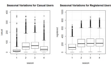
Figure 3 shows the variation in hourly demand for Casual, Registered, and All (Casual + Registered) users both for working days and on non-working days.

         Figure 3.          Hourly Demand for Casual, Registered and All Users on Working Days vs. Non-Working Days

 

 

From Figure 3, we see that demand on working days is driven primarily by registered users with spikes in demand and variability during peak hours.  On non-working days, registered users still account for more than half the demand, but casual users account for much of the variability.  Non-working days do not exhibit clear peak hours, with most of the demand spread over a wider duration between 1000h and 1900h.

The trends and patterns we have observed so far may trigger more questions.  For example, is it more meaningful to look at monthly variations rather than seasonal variations?  How do weather conditions play a part?  Visualizing the data is by decision trees may give us some insights.  Using the rpart package (Atkinson and Therneau, 2014) and plotted using the prp package (Milborrow, 2011), Figures 4 to 6 are decision trees that are produced by finding the best split that maximizes the difference in between-group sum-of-squares.  Only the first 3 to 4 layers of the decision trees were plotted to fit into this document.  Figure 4 shows the decision tree for hourly demand by registered users between 7 am and 7 pm.  The nodes contain the average hourly demand before each subsequent split as we go down the tree.  The branches are annotated with the conditions of each split.  In Figure 4, the tree mirrors the analysis we did with the box plots, with no real surprises.  Rentals by registered users spike at peak hours (i.e. 0800h, 1700h and 1800h) on working days, user growth from 2011 to 2012 accounts for significant variation in demand and there is a drop in demand during off peak hours in the months from Jan 2011 to Apr 2011. 

                                   Figure 4.          Decision Tree for Registered Users (7 am to 7 pm)

 

The decision tree for casual users is in Figure 5.  If we following the rightmost path along the tree, we can see that casual users tend to rent bikes between 1000h and 1900h, more so on non-working days and when temperature feels above 22 degrees.  The demand is also higher in 2012.  These observations are also consistent with those made earlier.

                                              Figure 5.          Decision Tree for Casual Users (Depth = 4)

It is interesting to delve further down the decision tree to observe how casual users behave.  Figure 6 is the subtree branching down from the rightmost leaf node in Figure 5.  This time, apart from printing the average hourly demand in the node, we also print the number of instances (n) for each node.  When we traverse this sub-tree by moving down two branches to the right, we notice that that casual users rent a lot less bikes if it was a public holiday compared to other non-working days (i.e. weekends) possibly because casual users tend not to come or stay in town during holidays.  We can also see in the rightmost subtree a drop in demand when the humidity is above 82 degrees possibly because it is much less comfortable to take a leisurely ride when it is humid. However, we should take this observation with some skepticism because there are only 3 instances in this terminal node.

                  Figure 6.          Sub-Tree for Casual Users from Rightmost Node in Figure 5

 

Note that this tree branches from the rightmost leaf node in Figure 4.  The month of December is missing because there were no hours in December 2012 for a non-working day where the temperature was more than 22 degrees.

A single decision tree is not only easy to interpret but can also serve as a model for prediction.  However, a single decision tree is prone to under-fitting when the depth is small, or overfitting when the depth is too high.  Nonetheless, we decided to include a decision tree as another baseline to compare against other algorithms.

C.                Algorithm Selection from first-pass modeling

The results of the first-pass modeling using 5 different algorithms are presented in Table 8.  The RMSLE scores were obtained from the Kaggle website when we submitted our predictions for the test set.  The rankings are based on the final leaderboard (https://www.kaggle.com/c/bike-sharing-demand/leaderboard), reflecting where each algorithm would have ranked out of the best submissions of 3,252 teams.  We can see that Gradient Boosting with decision trees and Random Forest produced much better results than the other algorithms.  The results confirm the observation by Hastie et al. (2009) that Boosting and Random Forest produce similar results with an RMSLE of 0.420 vs 0.424 respectively.  Even the single decision tree (0.546) performed better than Support Vector Regression (0.720) and Ridge Regression (0.6231).  This suggests that decision-tree methods are naturally more suited for this application.  Perhaps surprisingly, Support Vector Regression actually performed worse than Ridge Regression.

                          Table 8.  RMSLE and Ranking obtained by 5 different algorithms

The results were obtained by simply applying the algorithms directly to predict log(count) and by tuning the parameters for each algorithm to obtain their best results respectively.

While it is possible that the results of each algorithm can be improved further by spending more time on adjusting the parameters or by feature engineering, we decided to choose only the Gradient Boosting and Random Forest algorithms for further analysis and modeling since they appear to be better suited for this problem.

D.                Variable Importance FROM RANDOM FOREST

Gradient Boosting and Random Forest are ensemble methods that combine predictions from multiple decision trees in different ways to produce an often-better prediction.  However, the better prediction comes at a cost to interpretability.  While a single decision tree is easily interpretable, a sequence of 1000 boosted trees in Gradient Boosting or 500 random trees in Random Forest is difficult to interpret and visualize.  Fortunately, the Random Forest package in R allows us to calculate the importance of each factor in two ways (Liaw & Wiener, 2012).  The first measure (%IncMSE) is calculated by quantifying the average increase in mean squared error across the trees when the values of the variable in question are randomly permuted before making a prediction, compared to predictions made without random permutation (Strobl, Boulesteix, Zeileis, and Hothorn, 2007).  These predictions are made on out-of-bag samples (i.e. samples that were not selected during bagging for training the tree).  The second measure (IncNodePurity) is the total decrease in node impurities (i.e. total decrease in residual sum of squares) each time the variable in question is used for splitting a leaf node in the tree (Liaw & Wiener, 2012).  This is averaged across all the trees in the forest.  Tables 9 and 10 present the variable importance for registered users and casual users respectively.  Once again, we can see casual users are more affected by weather variables than registered users.

                                                  Table 9.  Variable Importance for Registered Users

This table was produced setting the importance option to TRUE in the randomForest R package and sorted by decreasing %IncMSE (i.e. increase in mean-squared error).

                                                  Table 10.         Variable Importance for Casual Users

 

Although the R package is able to estimate variable importance this way, it is difficult to interpret this importance quantitatively because each variable is different.  Strobl et al. (2007) assert that the approach used to calculate variable importance in the random-forest package is biased in favor of variables with many categories and continuous variables, and propose alternative methods to get a more accurate measure of importance.  We will nonetheless be using Tables 9 and 10 as a point of reference to perform feature selection to fine-tune the model.

E.                 DISCUSSION ON THE RMSLE EVALUATION FUNCTION

We discuss the impact of using root-mean-squared logarithmic error (RMSLE) as the evaluation metric.  Using the logarithmic-based calculation ensures that the errors during peak hours do not overshadow the errors made during off peak hours.  Table 11 gives us some insight to how an actual missed prediction affects the RMSLE.

                                             Table 11.         Missed Predictions vs. Logarithmic Error

Scenario	Actual demand (a)	Predicted demand (p)	Real error (a-p)	% error ((p-a)/a)	log actual log (a+1)	log predict (log (p+1))	Log error (log(a +1)-log(p+1))
1	0	1	1	NA	0.000	0.693	0.693
2	0	2	2	NA	0.000	1.099	1.099
3	2	3	1	50%	1.099	1.386	0.288
4	2	4	2	100%	1.099	1.609	0.511
5	5	6	1	20%	1.792	1.946	0.154
6	10	12	2	20%	2.398	2.565	0.167
7	100	120	20	20%	4.615	4.796	0.181
8	500	600	100	20%	6.217	6.399	0.182
9	1000	1200	200	20%	6.909	7.091	0.182
10	1000	1100	100	10%	6.909	7.004	0.095

 

A 20% over-prediction produces a consistent logarithmic error (0.154 � 0.182) when the actual demand ranges from 5 to 1000 (Scenarios 5 -10).  While this is desirable from a mathematical perspective, it is less meaningful from an economic perspective since a 20% miss during peak hours has a greater cost than at other times.  Similarly, missed predictions when actual demand is less than 5 could easily result in large logarithmic errors, as can be seen in the first four scenarios of Table 11.  For example, when the actual demand is 2 and the predicted demand is 4, the log error is 0.511 which is almost 3 times more serious than when the actual demand is 1000 and the predicted demand is 1200.  In fact, minimum actual count occurs often between midnight and 6 a.m.  Between 2 and 4 a.m., the hourly demand ranges from 0 to 66 while the median and average demand is 6 and 8.9 respectively.

To understand how this affects our results, we plot the absolute error in logarithmic demand against the actual count (Figure 7) when our gradient boosting model was used to predict a 20% validation set with 2177 instances. We notice that larger logarithmic errors are indeed being made when the count is low.  Furthermore there is a bias towards overestimation.  Beyond an actual count of 200, the absolute logarithmic error is mostly less than 0.182 or a 20% misprediction (see Table 11).

                                                          Figure 7.          Logarithmic Error vs. Actual Count

Left: raw logarithmic error / Right: absolute logarithmic error

The decision trees in Figure 8 present the same information, but offer a better quantitative feel of how the RMSLE score is affected by missed predictions when the demand is low.  In the tree on the left, the mean error in logarithmic demand is 0.3 when the count is less than 6.5 (177 cases), the mean error for the rest of the cases is a mere -0.03.  This drops to 0.16 for all other hours (1562 cases).  With the tree on the right, the absolute error is 0.32 when the actual demand is less than 54 (612 cases).  This drops to 0.15 when the predicted demand is more than 54 (1565 cases). 

               Figure 8.          Error in Logarithmic Demand vs Actual Count (Decision Tree)

 

From this analysis, we can conclude that RMSLE is not the most suitable evaluation metric if we are most interested in resource allocation when demand is high.  A weighted RMSLE may be a possible alternative, but for the competition and the main results of this thesis, we did use RMSLE.

F.                 MODEL FINE-TUNING USING THE RANDOM FOREST ALGORITHM

From Table 8, we saw that Random Forest and Gradient Boosting achieved similar performance.  Although Gradient Boosting is relatively faster, we found it much harder to tune and more prone to overfitting on this dataset than Random Forest.  Random Forest produced very stable cross-validation RMSLE (using more than 200 trees) once the best value of the number of variables to choose at each split was determined.  For the rest of this thesis, we focused on Random Forest as the algorithm for further experiments to improve our modeling.  We used 10-fold cross-validation RMSLE and test-set RMSLE to evaluate our experiments.  We also provide the ranking for each model by submitting the results to the Kaggle website after the competition has ended since rankings are constantly in flux when the competition is still open.  The findings are described in the following paragraphs.

1.                  Predicting Casual and Registered demand separately

As we saw in our data visualization (Figure 3), casual and registered users exhibit different behavior, so it was natural to check if creating two sub-models to predict the demand from each group would improve performance.  We performed a 10-fold cross validation with the training set to obtain the cross-validation RMSLE, and obtained the test-set RMSLE by submitting the predictions to the Kaggle website.  The results are presented in Table 12.   We can see that there is indeed an improvement in performance.  From this point on, we will only be using two sub-models for further performance tuning.  We will refer to this our base model.

         Table 12.         Effect of using separate models to predict registered and casual users vs. using a single model to predict count

 

2.                  Feature selection

As discussed in Chapter III, there are obvious correlations in several input variables (e.g. weekday and working day).  There is therefore a possibility that prediction accuracy can be improved by selecting a subset of the number of input variables.  The selections could be different for casual and registered users.  Even with a relatively small number of variables (12), the number of combinations to build different models grows very quickly, so we referred to variable importance in Tables 9 and 10, and applied some heuristics to limit the exploration space.  From the initial 12 variables, we eliminated windspeed and holiday as factors because they were ranked lowest in variable importance (%IncMSE) for both registered and casual users (see Tables 9 and 10).  From the remaining 10 variables, we selected 6 variables to be included in all subsets based on their %IncMSE values for registered and casual users (see Tables 9 and 10) while avoiding variables that were strongly correlated.  We selected all combinations of the last 4 variables.  Table 11 presents ourvariable-selection scheme.  

                                                                    Table 13.         Variable-Selection Scheme

 

The variable-selection scheme in Table 13 has 16 different subsets requiring 16 cross-validation runs.  We chose to perform 5-fold cross-validation with 200 trees.  Table 14 presents the RMSLE for the sub-models (casual and registered) and the combined model (count) for the 16 different variable subsets.  The best performance (RMSLE = 0.317) was achieved by selecting (month + weather) or (month + weather + season) along with the 6 core variables (year, working day, day, hour, atemp, and humidity).  Unfortunately, none of the combinations produced significantly better results than the base model (RMSLE = 0.319).   From Table 12, we can see that the RMSLE for casual is significantly higher than for registered, but the overall RMSLE is very close to that for registered users, due likely to the fact that there are a lot more registered users than casual users.  There are also more than twice as many non-working days than working days.  It is on these days that registered users greatly outnumber casual users (see Figure 3).

                                                              Table 14.          Results of Cross Validation

Variables included in all runs	month	season	weather	temp	RMSLE (casual)	RMSLE (registered)	RMSLE (count)
year, working day, day, hour, atemp, humidity					0.550	0.392	0.389
	x				0.498	0.330	0.330
		x			0.514	0.338	0.338
			x		0.534	0.376	0.372
				x	0.539	0.385	0.382
	x	x			0.495	0.329	0.329
	x		x		0.486	0.318	0.317
	x			x	0.496	0.330	0.330
		x	x		0.501	0.324	0.324
		x		x	0.511	0.337	0.337
			x	x	0.524	0.372	0.368
	x	x	x		0.483	0.317	0.317
	x	x		x	0.494	0.331	0.331
	x		x	x	0.486	0.320	0.319
		x	x	x	0.499	0.325	0.325
	x	x	x	x	0.485	0.321	0.320

The 6 variables in the first column are included in all 16 subsets.  A cross under a variable column means that the variable is included in the subset of features.

The findings from the cross-validation runs did not justify reducing the number of variables, although there is still a possibility that a reduced set could improve the performance with respect to the test set.  In fact, our best result for the test set was obtained by using a set of variables (see Table 15) that were in a script published on the Kaggle website, which we used as starter code for running our own experiments.  There was no mention by the author of how this set of variables was selected, but we obtained a test-set RMSLE of 0.3852 for a ranking of 141^st out of 3252 teams.  Since it was our best test-set prediction, we used this as our final submission to the competition. However, for the rest of thesis, we elected to keep the entire set of 12 variables to continue with further experiments.

                             Table 15.         Variables that Produced our Best Test-Set RMSLE

The variables were used in the script published on https://www.kaggle.com/bruschkov/bike-sharing-demand/0-433-score-with-randomforest-in-r/code

3.                  Adding Features to Improve Prediction for Wee Hours

As discussed earlier, the RMSLE tends to be high when the actual count is low.  This occurs most often during hours between midnight and 5 a.m.  In order to improve prediction during these hours, we added a feature called wee_hours which is a binary variable that has value 1 for hours between midnight and 5am and 0 otherwise.  We further hypothesized that the demand for bicycles during hours before midnight and wee hours is especially sensitive to whether it was a working day the following day or the previous day.  Therefore, we added two other binary variables work_tmr and work_ytd as features which simply mirror the values of the binary variable working_day for the following day and the previous day respectively.  We manually added the boundary cases for 1 Jan 2011 and 31 Dec 2012.  Table 16 presents the results of the experiment.  With the new features, we managed to reduce RMSLE for both the cross-validation set and the test set.

               Table 16.         Adding Features to Improve Predictions during Wee Hours

 

4.                  Accounting for Trends (Moving Average and Week Number)

As described in Chapter III, including the moving average of demand as a factor may improve prediction since it would help account for multiday trends like user growth and seasonal variations.  We decided to take the average hourly demand over the past 7 days as a factor.  The computation of the 7-day average demand (MA7) was complicated by the fact that our training set was not continuous.  This was overcome by using a first model to predict the demand and using it as a proxy to estimate MA7, as described in Chapter III.  Table 17 presents the results from this approach.  The introduction of MA7 improved the results for the 10-fold cross validation error from 0.319 to 0.314.  Although the improvement was small, it was consistent across the 10 different cross-validation folds.  Unfortunately, this resulted in a very slight increase in test-set error from 0.41274 to 0.41426.  However, given the fact that the test-set error can exhibit variations of about �0.005 when a different random set is used, this increase is not statistically significant.

As a next step, we added a new numerical feature called week_number to represent the number of weeks lapsed with respect to 1 Jan 2011 to experiment if it complements MA7 in modeling demand growth.  As a fictive example, a large number of new kiosks or bikes may have been added in Week 30.  Our previous model might not detect such changes because year, month and day have all been modeled as categorical variables.  Adding week_number again improved the cross-validation RMSLE consistently over the 10 folds, but resulted in an increase in RMSLE in the test set, possibly due to overfitting (see Table 17).

           Table 17.         Adding Features to Account for Trends (Moving Average and Week Number)

 

5.                  Combining the New Features

We experimented with combining the new features from the two preceding sections with the base model.  The results are presented in Table 16.  The best result for cross-validation RMSLE was obtained by adding MA7 and Week Number as features.  However, this combination produced the worst test-set RMSLE.  On the other hand, the best results for test-set RMSLE was obtained by combining the Base Model with the Wee Hour Features (i.e. wee_hours, work_tmr, and work_ytd).  This combination had the second poorest RMSLE from cross-validation.

                                         Table 18.         Combining New Features with Base Model

 

V.               Chapter 6: Conclusion

 

A.                SUMMARY OF FINDINGS

This thesis explored a range of machine-learning algorithms to predict hourly demand in a bike-sharing system.  We found tree-based regression algorithms to perform the best among the tested algorithms.  Specifically, the Random Forest and Gradient Boosting algorithms produced the best results when applied to the test set.  The Random Forest algorithm was easier to tune as the performance tended to be more stable when parameters are tweaked.  Tuning the Gradient Boosting algorithm required more experimentation to find the parameter settings that produced the best results.  Gradient Boosting was also prone to overfitting on this dataset.  However, Gradient Boosting was significantly faster than Random Forest once the right settings were found.

In the following phase of the study, we fine-tuned a model using the Random Forest algorithm.  From factor importance metrics produced by Random Forest, we confirmed our intuition and statistical analysis that the demand from casual users and registered users were driven by different factors.  It made sense to train two different models to predict the demand for each group.  This improved the results for both cross-validation RMSLE and test-set RMSLE.  All subsequent experimentation was based on this two sub-model approach, which we call the base model (10-fold cross-validation RMSLE = 0.319, test-set RMSLE = 0.42388)

Next, we experimented with feature selection to find out if a subset of variables would produce better results than the full set, due to correlations between many of the features.  We used 5-fold cross-validation to try out 16 different combinations of the 12 original features.  The 16 combinations were chosen by retaining 6 of the most important features, eliminating the 2 least important, and a full factorial combination of the 4 remaining features.  The cross-validation results did not look promising, with only 2 of the 16 combinations producing any improvement and it was marginal (RMSLE = 0.317).  Interestingly, we managed to get our best test-set RMSLE of 0.3852 by using a different subset of variables from a published script that we forked.  However, since we did not understand how the variables were selected, we elected to continue experimenting with all 12 of the original features.

In further experiments, we added three features (wee_hours, work_ytd, and work_tmr) to improve prediction for hours between midnight and 5 a.m., which improved the test-set RMSLE (0.40665).  In a parallel experimentation, we also added the 7-day moving average for hourly demand and week number as additional features to account for temporal dependences.  This improved the 10-fold cross-validation RMSLE to 0.308.  However, there was discrepancy between improvements in cross-validation RMSLE and test-set RMSLE.

B.                 LESSONS LEARNED

We found Random Forest and Gradient Boosting to be suitable algorithms to predict hourly demand in similar resource-sharing systems.  Random Forest achieved very good results with minimal tuning and is a good candidate for modeling similar datasets (e.g. subway usage and traffic flow).  Depending on the accuracy required, it may be profitable to build separate models for distinctly different groups of users (e.g. casual and registered), although models that predict the aggregate count directly did fairly well.

From an economic perspective, we should be most concerned with missed predictions during peak hours.  However, RMSLE as a measure of performance overcompensates for errors made during off-peak hours.  We recommended using an alternative error measurement such as a weighted RMSLE to accurately reflect economic objectives, or simply building models solely for peak-hour traffic.

Beyond the basic Random Forest and Gradient Boosting models, we performed several experimentations to try to boost our ranking from 373^rd out of 3000 teams.  We tried eliminating features (feature selection) systematically using cross-validation error but did not find good candidate features.  However, our best-performing model in terms of test-set RMSLE was obtained fortuitously by using a set of variables from a published script which we forked.  This discrepancy between cross-validation error and test-set error re-emerged when we tested different ideas for feature engineering and saw decreases in cross-validation error that caused increases in test-set error in some cases.  This could be caused by overfitting due to model complexity, and was possibly exacerbated by the way the test set was sampled in this competition.  Our test set was carved out from the last 9 � 12 days of each month and it is possible that some patterns in the test set were never encountered in the training set.  We recommend using random sampling to form training sets to minimize this risk.

C.                RELATED WORK

Prediction models such as those addressed in this thesis have several possible applications.  Kolka (2011) discusses how to prescribe the number of bicycles to be repositioned (by trucks) from one station to another to minimize shortage based on demand forecast.  However, this would require forecasting models to be built at a higher granularity (i.e. per station or neighborhood) rather than at the aggregate level.  Fanaee-T and Gama (2013) studied the use of predictor ensembles as detectors to automatically flag outliers (i.e. spikes in demand) in order to detect anomalous events.  Froehlich, J., Neumann, J., & Oliver, N. (2009) used bike-sharing data to glean insights on city dynamics from a cultural and space-time perspective.  The lessons learned from this thesis can also be applied to similar datasets to predict demand for other forms of public transportation and support operations planning.

THIS PAGE INTENTIONALLY LEFT BLANK

List of References

Atkinson, E., & Therneau, T. (2014) rpart: Recursive partitioning and regression trees.

Belissent, J. (2010). Getting clever about smart cities: New opportunities require new business models. Forester Research.

Breiman, L. (2001). Random forests. Machine learning, 45(1), 5-32.

Caruana, R., & Niculescu-Mizil, A. (2006, June). An empirical comparison of supervised learning algorithms. In Proceedings of the 23rd international conference on Machine learning (pp. 161-168). ACM.

Dimitriadou, E., Hornik, K., Leisch, F., Meyer, D., & Weingessel, A. (2008). Misc functions of the Department of Statistics (e1071), TU Wien. R package, 1-5.

Fanaee-T, H., & Gama, J. (2013). Event labeling combining ensemble detectors and background knowledge. Progress in Artificial Intelligence, pp. 1-15.

Freund, Y., & Schapire, R. E. (1997). A decision-theoretic generalization of on-line learning and an application to boosting. Journal of computer and system sciences, 55(1), 119-139.

Friedman, J. H., Hastie, T., & Tibshirani, R. glmnet: lasso and elastic-net regularized generalized linear models, 2010b.

Froehlich, J., Neumann, J., & Oliver, N. (2009). Sensing and Predicting the Pulse of the City through Shared Bicycling. In IJCAI (Vol. 9, pp. 1420-1426).

Ridgeway, G. (2012). Generalized Boosted Models: A guide to the gbm package.

Hastie, T., Tibshirani, R., & Friedman, J. (2009). The Elements of Statistical Learning.

Hoerl, Arthur E., and Robert W. Kennard. Ridge regression: Biased estimation for nonorthogonal problems. Technometrics 12.1 (1970): 55-67.

Kaggle Inc. (2014). Bike Sharing Demand � Forecast use of a city bikeshare system. Retrieved Jul 28, 2015 from https://www.kaggle.com/c/bike-sharing-demand

Kolka, O. (2011). Management of Stock Levels in a Bike-Sharing System (Doctoral dissertation, TEL AVIV UNIVERSITY).

LDA Consulting. (2013). 2012 capital bikeshare member survey report executive summary.

Liaw, A., & Wiener, M. (2012). Package �randomForest�. R Package.

Milborrow, S. (2011). rpart.plot: Plot rpart Models. An Enhanced Version of plot.rpart., 2011. R Package.

Opitz, D., & Maclin, R. (1999). Popular ensemble methods: An empirical study. Journal of Artificial Intelligence Research, 169-198.

Shaheen, S. A., Martin, E. W., Chan, N. D., Cohen, A. P., & Pogodzinski, J. M. (2014). Public Bikesharing in North America During a Period of Rapid Expansion: Understanding Business Models, Industry Trends & User Impacts.

Smola, A. J., & Sch�lkopf, B. (2004). A tutorial on support vector regression. Statistics and computing, 14(3), 199-222.

Strobl, C., Boulesteix, A. L., Zeileis, A., & Hothorn, T. (2007). Bias in random forest variable importance measures: Illustrations, sources and a solution. BMC bioinformatics, 8(1), 25.

Vapnik V., Golowich S., and Smola A. 1997. Support vector method for function approximation, regression estimation, and signal processing. In: Mozer M.C., Jordan M. I., and Petsche T. (Eds.) Advances in Neural Information Processing Systems 9, MA, MIT Press, Cambridge. pp. 281�287.

Vapnik V. and Lerner A. 1963. Pattern recognition using generalized portrait method. Automation and Remote Control, 24: 774�780.

 

 

 

THIS PAGE INTENTIONALLY LEFT BLANK

 

initial distribution list

1.         Defense Technical Information Center

            Ft. Belvoir, Virginia

 

2.         Dudley Knox Library

            Naval Postgraduate School

            Monterey, California