Associating Drives Based on ��������������������������������������������Their Artifact and Metadata Distributions

Neil C. Rowe1

¹ Computer Science, U.S. Naval Postgraduate School
ncrowe@nps.edu

Abstract. Associations between drive images can be important in many forensic investigations, particularly those involving organizations, conspiracies, or contraband.� This work investigated metrics for comparing drives based on the distributions of 18 types of clues.� The clues were email addresses, phone numbers, personal names, street addresses, possible bank-card numbers, GPS data, files in zip archives, files in rar archives, IP addresses, keyword searches, hash values on files, words in file names, words in file names of Web sites, file extensions, immediate directories of files, file sizes, weeks of file creation times, and minutes within weeks of file creation.� Using a large corpus of drives, we computed distributions of document association using the cosine similarity TF/IDF formula and Kullback-Leibler divergence formula.� We provide significance criteria for similarity based on our tests that are well above those obtained from random distributions.� We also compared similarity and divergence values, investigated the benefits of filtering and sampling the data before measuring association, examined the similarities of the same drive at different times, and developed useful visualization techniques for the associations.

 

This paper appeared in the Proceedings of the 10^th EAI International Conference on Digital Forensics and Computer Crime, New Orleans, LA, September 2018.

Keywords: Drives, Forensics, Link Analysis, Similarity, Divergence, Artifacts, Metadata.

1               Introduction

Most investigations acquire a set of drives.� It is often important to establish associations between the drives as they may indicate personal relationships and downloading patterns that can provide leads.� Such link analysis has become an important tool in understanding social networks.� Methods of digital forensics now allow us to do link analysis from drive features and artifacts.� Knowing that two drives share many email addresses, files, or Web-page visits establishes a connection between them even before we know exactly what it is.� Such associations are important in investigating criminal conspiracies and terrorists, intellectual-property theft, propagation of malware or contraband, social-science research on communities, and in finding good forensic test sets.�

However, there are big challenges to forensic link analysis from drive data. �One is the large amount of irrelevant data for most investigations, especially in files that support software [10].� A second problem is determining how best to establish associations between drives.� Some clues are more helpful for further investigation (such as email addresses), some are harder to extract (such as all words in file names, or worse, all words within files), and some are harder to compare (such as personal-file names).

This work attempted to answer these challenges by investigating 18 kinds of relatively easily calculable clues that could relate drives.� They include both forensic artifacts obtained by scanning tools, such as email addresses and phone numbers, and metadata obtained from file directories, such as file sizes and words in file names.� Most are routinely collected by tools such as SleuthKit.� Processing can be made faster by filtering out data unlikely to be of forensic interest or by sampling.

This work tested association methods on a large corpus of drives using cosine similarity and divergence, and tried to establish significance thresholds.� Similarity or divergence do not prove causation or communication since two associated drives may have obtained data from a common source. �However, associations suggest structure in a corpus and that can be interesting in its own right.

This work is empirical research.� Empirical methods may be rare in digital forensics, but are common and accepted in other areas of science and engineering.� Empirical research can justify methods and algorithms by tying them to careful observations in the real world.

This paper will first review previous work.� It then introduces the corpori studied, the clues used to compare drives, and formulae used for comparison.� It then presents several kinds of results and makes some recommendations for associating drives.

2               Previous work

Comparing drive data was first explored in [8] under the term "cross-drive analysis".� That work compared email addresses, bank-card numbers, and U.S. social-security numbers to relate drives.� This work has not been much followed up although it has been integrated into a broader investigative context in [11], combined with timeline analysis in [14], and applied to malware detection in [6].� Hashes on regular partitions of drive images [22] can relate all the data on drives including unallocated storage, but they are sensitive to variations in placement of data and their computation is time-consuming.� Scanning drives for particular keywords [7] is also time-consuming.� It would thus seem useful to evaluate the original idea of cross-drive analysis with a systematic approach to possible features and methods for comparison.

Previous work has measured similarities between documents for aiding online searches.� That work focused heavily on word and word-sequence [7] distributions of documents, with some attention to weighting of word values and measuring the "style" of a document [13].� Much of this work uses the cosine similarity and the Kullback-Leibler divergence to be discussed; some uses the Jaccard distance and its variants [12]; some uses latent semantic indexing; and some uses the Dirichlet mixture model [20].� Although we used the Jaccard formula previously, it is crude because it treats all words as equally important.� Latent semantic indexing only works for words with a rich semantics.� The Dirichlet mixture model assumes the data is a superposition of distinct processes, something not often true for digital-forensic data.� Document-comparison methods have been generalized to other kinds of data as in measuring similarity of files to known malware [21].� Generalization is important for digital forensics because many distinctive features of drive images such as IP addresses and file sizes are not words.

Similarity can also be based on semantic connections, but that is mainly useful for natural-language processing and we do not address it here.� Note that similarity of drives is different from the similarity between artifacts on the same drive suggested by colocation and format similarity, a lower-granularity problem addressed elsewhere [18].�

Usually the goal of analysis of forensic links is to build models of social networks [26; 5; 25].� Degree of association can be thresholded to create a graph, or the inverse of similarity can be used as an approximate distance and the points fitted to a metric space as we will discuss.� Associated data can also be aggregated in a forensic integration architecture [15] to enable easier systematic comparison.

3               Data used in experiments

This work used five corpori.� The main one was images of 3203 non-mobile drives of the Real Data Corpus (RDC) [9], a collection obtained from used equipment purchased in 32 non-US countries around world over 20 years, of which 95% ran the Windows operating system.� A second corpus was the 411 mobile devices from the RDC, research sponsors, and our school.� A third corpus was 236 randomly selected classroom and laboratory computers at our school (metadata and hash values only).� In total we had 3850 images of which 977 had no identifiable operating system though possibly artifacts.� Artifact data was obtained for the RDC with the Bulk Extractor open-source tool [4] for email, phone, bank-card, GPS, IP-address, URL, keyword-search, zip-file, and rar-file information.

The Mexican subcorpus of the RDC, 177 drives in eight batches purchased in Mexico, was analyzed to provide the more easily visualized results shown later in this paper.� Also studied was the separate M57 patent corpus [24], a collection of 83 image "snapshots" over time for a set of machines with scripted usage.� Its snapshots on different days provide a good test of high-similarity situations.� All five corpori are publicly available under some access restrictions.

4               Measuring drive associations

4.1           Clues to associations

The experiments described below focused on clues from artifacts and metadata that are often routinely calculated in forensic investigations and do not require additional processing.� Artifact clues (the first 11 below) were obtained with Bulk Extractor tool, and metadata clues (the remaining 7) were obtained with the Fiwalk open-source tool now included with SleuthKit (www.sleuthkit.org).� Experiments were done both with the raw set of clues and with the subset after filtering to eliminate the likely uninteresting ones.� Filtering methods are described below.� In general, filtering of artifacts tried to eliminate vendor and organization contact data, fictional data, artificial data, and ambiguous data (such as "mark field" as a personal name).� Filtering of metadata tried to eliminate software-associated files not containing personal information.� These filtering criteria are appropriate for criminal and intelligence (but not malware) investigations.� The clues were:

�         Em: Email addresses, found by Bulk Extractor's "email" plugin.� Filtering was done using a stoplist (exclusion list) of 500,000 addresses found by NIST in their National Software Reference Library, plus filtering of clues whose rating was under a threshold by our Bayesian rating scheme [18] using factors such as the appearance of known personal names, type of domain, and number of drives on which the name was found.� Bayesian parameters were calculated from a manually labeled training set.

�         Ph: Phone numbers, found by Bulk Extractor's "phone" plugin.� Bayesian filtering [17] excluded candidates based on factors such as informational area codes, artificiality of the numbers, and number of drives having that number.

�         Pn: Personal names, found by our methods using dictionary lookup of known personal names and regular expressions applied to Bulk Extractor�s �context� output [17].� Bayesian filtering eliminated candidates based on factors such as delimiters, use of dictionary words, and adjacency to email addresses.�

�         Sa: Street addresses, found using regular expressions on Bulk Extractor�s "context" argument.� Bayesian filtering used factors of the number of words, position in the argument, suitability of the numbers for addresses, capitalization of the words, length of the longest word, number of digits in the numbers, use of known personal names, use of words frequently associated with streets like "Main", "street", and �rd�, use of "#", and membership in a stoplist of 2974 adverbs, conjunctions, prepositions, and common computer terms.

�         Bn: Numeric strings that could be bank-account numbers, found using Bulk Extractor's "ccn" plugin. �Error rates were high.� Filtering excluded numbers not well delimited.

�         Gp: Formatted GPS data found by Bulk Extractor's "gps" plugin.� There were only a few instances in our corpori.

�         Zi: Zip-compressed files found by Bulk Extractor.� They are a weak clue to drive similarity since there are many frequently-seen zip archives. Filtering excluded those on 10 or more drives.

�         Ra: Rar-compressed files found by Bulk Extractor, handled similarly to zip-compressed files.

�         Uw: Words in the file names of Web links found by Bulk Extractor's "url" plugin.� We did not consider numbers and words of directory names because they usually indicate infrastructure.� Filtering excluded words in the Sa-clue stoplist.

�         Ks: Keywords in searches found by Bulk Extractor�s �url_searches� plugin (26% of which were from the browser cache).� Filtering excluded those occurring on 10 or more drives.

�         Ip: Internet IP addresses [2].� Filtering excluded addresses on ten or more drives. �However, they have more to do with software and local configurations than URLs do, and thus do not help as much to identify the similar user activity which matters more in most forensic investigations.

�         Ha: MD5 hash values computed on files.� Filtering excluded files based on ten factors described below.

�         Fn: Words in the file names on drives.� Filtering used the ten factors.

�         Ex: File extensions on the drive including the null extension.� Filtering used the ten factors.

�         Di: Immediate (lowest-level) directory names on the drive (with the null value at top level).� Filtering used the ten factors.

�         Fs: Logarithm of the file size rounded to the nearest hundredth.� Comparing these suggests possible similar usage.� Filtering used the ten factors.

�         We: Week of the creation time on the drive.� Its distribution describes the long-term usage pattern of the drive; [1] and [14] argue for the importance of timestamps in relating forensic data.� Filtering used the ten factors.

�         Ti: Minute within the week of the creation time.� This shows weekly activity patterns.� Filtering used the ten factors.

U.S. social-security numbers and other personal identification numbers were not included because our corpus was primarily non-US and the formats varied.� Sector or block hashes [22] were not included because obtaining them is very time-consuming and results in large distributions.� As it was, comparing of hash values on full files took considerably more time than analysis of any other clues.

Filtering of the metadata clues used ten negative criteria developed and tested in [16]: hash occurrence in the National Software Reference Library (NSRL), occurrence on five or more drives, occurrence of the file path on 20 or more drives, occurrence of the file name and immediate directory on 20 or more drives, creation of the file during minutes having many creations for the drive, creation of the file during weeks with many creations for the corpus, occurrence of an unusually common file size, occurrence in a directory whose other files are mostly identified as uninteresting by other methods, occurrence in a known uninteresting directory, and occurrence of a known uninteresting file extension.� Filtering also used six overriding positive criteria indicating interestingness of a file: a hash value that occurs only once for a frequent file path, a file name that occurs only once for a frequent hash value, creation in an atypical week for its drive, an extension inconsistent with header analysis, hashes with inconsistent size metadata, and file paths including words explicitly tagged as interesting such as those related to secure file erasure.� Files were filtered out if either they matched NSRL hashes or matched at least two negative criteria and none of the positive criteria.� Applying the criteria provided a 77.4% reduction in number of files from the RDC (with only 23.8% due to using NSRL) with only a 0.18% error rate in failure to identify potentially interesting files, as estimated by manual investigation of a random sample [16].�

Table 1 gives counts of the clues found in our main corpus of the RDC, mobile, and school drives.� The first column gives the raw count of the clue, the second column the count after the filtering described, and the third column the number of drives with at least 10 different values of the clue (our threshold for sufficient data for comparison). The fourth column counts the sum of the number of distinct clue values per drive, meaning that it counts twice a clue on two drives but once a clue twice on a single drive.

�

Table 1. �Counts of clues found on drives in our main corpus of 3850 drives.

Clue type	Count in our full corpus	Filtered count in our corpus	Number of drives having ≥ 10 values	Sum of distinct values over all drives in our filtered corpus
Email addresses (Em)	23,928,083	8,861,907	2,063	7,646,278
Phone numbers (Ph)	2,686,169	1,641,406	1,310	1,393,584
Personal names (Pn)	11,821,200	5,270.736	2,008	2,972,767
Street addresses (Sa)	206,506	135,586	782	88,109
Bank-card numbers (Bn)	6,169,026	5,716,530	671	332,390
GPS data (Gp)	159	159	4	121
Zip-compressed files (Zi)	11,993,769	4,218,231	1,302	3,886,774
Rar-compressed files (Ra)	574,907	506,722	654	382,367
Words in file names of Web� links (Uw)	1,248,356	204,485	981	7,631
Keyword searches (Ks)	849,894	769,520	830	661,130
IP addresses (Ip)	51,349	50,197	168	45,682
File hashes (Ha)	154,817,659	8,182,659	2,477	2,091,954
Words in file names (Fn)	19,095,838	6,178,511	2,567	759,859
File extensions (Ex)	1,003,609	422,638	2,288	27,810
Immediate directories (Di)	3,332,261	653,212	2,094	107,808
File size ranges (Fs)	2,275,412	1,671,392	2,731	2,003
File creation week (We)	577,035	254,158	1,906	1,749
File creation minute within week (Ti)	252,786	195,585	2,080	169

4.2           Measuring similarities and divergences

Document comparison methods use a variety of association formulae.� This work tested two of the best-known, the term-frequency inverse-document-frequency (TF-IDF) cosine similarity and the Kullback-Leibler divergence.� We interpret a "document" as the set of clues on a drive of a particular type, e.g. the set of email addresses on a drive, so to compare drives we compare clue distributions (histograms) per drive.� If �means the similarity of drives i and j, k is a clue-value number out of M possible clue values, �is the count of clue value k on drive i, �is the number of drives on which clue value k appears, and �is the classic inverse document-frequency weight for D drives total ([8] used a rarely-used logarithm-free formula) , the cosine-similarity formula is:

 

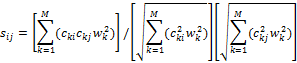
This ranges between 0 and 1 for nonnegative data such as counts.� Drives have considerably diversity on most of the clues investigated, so cosine similarities close to 0 are common for random pairs of drives.� An average similarity between two drives can be computed over all their similarities on clues.� However, similarities on different clues do mean different things and it can important to distinguish them.

Hash values on files are the most time-consuming of the clues on which to compute similarity since there are so many.� Computation time can be reduced by removing the hash values that occur on only one drive, about 61.2% of our main corpus, after counting them.� This count should be included in the denominator of the formula, but does not affect the numerator.

[23] notes that cosine similarity despite its popularity does not satisfy intuitive notions of similarity in many cases since it is symmetric.�� Asymmetric similarity would make sense for a drive having many downloads from a larger drive so a larger fraction of the smaller drive is shared.� So this work calculated an asymmetric measure of entropy-based Kullback-Leibler divergence on the clue distributions per drive, defined where �is is the total count of the first distribution and �is the total count of the second distribution as:

 

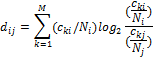
Divergence is smaller for larger similarities in a rough inverse relationship.� The formula is only meaningful when comparing clue values that the two distributions share, as we are computing for each value on drive j the similarity of its count to the count on drive i.� Thus �should be defined as the total count on drive i of items also on drive j.

Since divergence is directional, the minimum of the divergences in the two directions provides a single consensus value of association since the smaller divergence indicates the stronger association.� Also note that similarity and divergence are only meaningful with sufficient data, so at least 10 distinct clue values on each drive were required to compare two drives in our experiments.

5               Results

5.1           Comparing similarity and divergence

A large cosine similarity generally means a low divergence, and vice versa, so a question is to what degree they measure different things.� However, attempts to fit a formula from one to the other were unsuccessful with our data for the weighted average similarity and the weighted average divergence of the clues.� We tried the simplest possible formulae that could apply to an inverse relationship: , , , , and �; in each case a better least-square fit was obtained from .� We interepret this as meaning that similarity and divergence in general measure different things for our data, and it is useful to compute both.� However, the fit did vary with clue.� On the filtered data, the Pearson correlation coefficient between similarities and divergences was 0.744 for phone numbers, 0.679 for street addresses, and 0.659 for email addresses, but 0.451 for personal names and 0.332 for hash values.� The last makes sense because divergence rates highly the strong subsetting relationships between drive files whereas similarity does not.

5.2           Clue counts per drive

Histograms can be computed on the number of clue values per drive.� Many of these histograms approximated normal curves when the logarithm of clue count was plotted against the logarithm of the number of drives, but with an additional peak on the left side representing drives mostly lacking the clue.� Exceptions were for street addresses (uniform decrease with no peak) and time within the week (two peaks at ends of the range), the latter probably reflecting the difference between servers and other machines.

5.3           Significance tests of clue similarity

An important question is the significance of values of cosine similarity.� Figure 1 shows average similarities for the 10 artifact clues and Figure 2 shows average similarities for the 8 metadata clues, broken down by corpus.� The filtering was described in section 4.1; GPS data was insufficient and was excluded.� Two controls were obtained by taking 5000 random samples from the distribution of each of the clue values over all drives with sample sizes approximating the distribution of clue counts over all drives.� Thus the controls represent similarity values of completely uncorrelated random drives of the same total sizes as our corpus.� Results were similar for divergences but inverted.

The corpori show significantly more correlation than the controls, especially the school computers since they are centrally managed.� The average observed similarities in our corpori are so far above the controls that they are definitely significant even lacking ground truth about drive associations.� Note also that unfiltered data shows more similarities than the filtered data, most noticeably for file size (Fs) and file name (Fn), likely due to its larger number of spurious correlations.� Note also that filtering does not affect all clues equally.

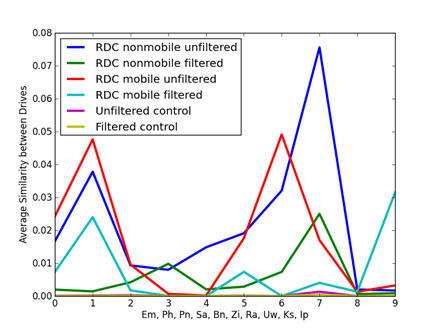
Figure 1: Average similarities for artifact clues.

 

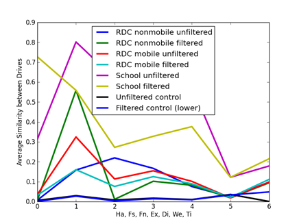
Figure 2: Average similarities for metadata clues.

 

The variances of the average similarities were significantly larger than the means, due to the large number of random pairs that had zero similarity.� Thus the similarity distributions are not Poisson.� Nonetheless, we can provide significance thresholds for similarity for each of the 18 clues by taking three standard deviations above the mean (Table 2), a standard statistical significance threshold.� This table is based on the RDC data, which should be a good model for many broad corpori because of its diversity.� The first two rows give thresholds for unfiltered distributions, and the last two for filtered distributions.�

 

Table 2: Recommended thresholds of significance for similarity between drives, for abbreviations defined in section 4; �UF� means unfiltered data and �F� means filtered data.

 

Table 3 shows average similarity by country code over all clues, a useful inverse measure of the diversity of our acquired drives by country.� Ratios of average similarities of metadata clues for undeleted versus deleted files were 1.304 for Fn, 1.471 for Ex, 1.202 for Di, 1.121 for Fs, 0.454 for We, and 0.860 for Ti.� So file deletion status mattered too for metadata clues; artifact clues were rarely within files.

 

Table 3: Average similarities as a function of the most common country codes.

 

5.4           The effects of sampling on similarities

When the primary goal is to find drive pairs with high similarities, processing time can be reduced by comparing random samples of the clues on the drives.� Table 4 shows the average effects over five random samples, each with sampling rates of 0.3, 0.1, and 0.03, on the similarities of our filtered RDC corpus for three artifact clues and three metadata clues.� Sampling generally decreased the similarities of drives and effects showed little variation between samples.� The artifact clues and file name words were more sensitive to sampling rates due to the smaller counts in their distributions.� Judging by this table, a 0.3 sampling rate will obtain 80% of the original similarity for many clues and should be adequate; file extensions, however, could be accurately sampled at a much lower rate.

�

Table 4: Average effects of random sampling on similarities of particular clues.

Clue	Sampling rate	Mean original similarity	Mean similarity of samples	Standard deviation of samples
Email address (Em)	0.3	0.00063	0.00047	0.00002
	0.1		0.00034	0.00002
	0.03		0.00024	0.00001
Phone number (Ph)	0.3	0.00070	0.00053	0.00001
	0.1		0.00040	0.00002
	0.03		0.00033	0.00003
Personal name (Pn)	0.3	0.00444	0.00380	0.00005
	0.1		0.00321	0.00007
	0.03		0.00256	0.00005
File extension (Ex)	0.3	0.13435	0.14290	0.00051
	0.1		0.14812	0.00069
	0.03		0.14856	0.00083
File name (Fn)	0.3	0.02394	0.02127	0.00007
	0.1		0.01684	0.00009
	0.03		0.01191	0.00008
File size (Fs)	0.3	0.19609	0.19098	0.00068
	0.1		0.16597	0.00049
	0.03		0.13258	0.00091

5.5           Correlations between clue similarities

Pearson correlations were measured between the similarities of different clues as a measure of clue redundancy.� Table 5 shows the results for main corpus without filtering, excluding GPS, bank-card, and rar files which did not occur frequently enough to be reliable in this comparison, and excluding drives for which there was no data for the clue.� The metadata clues (the last seven) were more strongly inter-associated than the artifact clues, though there was a cluster for email addresses (Em), phone number (Ph), personal names (Pn), and (interestingly) zip files (Zi).� The redundancy between the metadata clues suggests if we had to choose one, we should compare file extensions since they are easiest to extract and require little space to store.� Similarly, the weaker redundancy between the artifact clues suggests we compare email distributions because they are frequent artifacts, are easy to collect with few errors, and require little space to store.� Of course, each investigation can assign its own importance to clues, as for instance an investigation of a crime in a business might assign higher importance to phone numbers.� Note that IP addresses were uncorrelated with the other clues, suggesting that using them for link analysis [2] rarely reveals anything for unsystematically collected corpori like the RDC, and this is likely true for the closely associated MAC addresses as well.� As for processing times for clues, the times in minutes on a Gnu Linux 3.10.0 64-bit X86 mainframe for the total of extraction and comparison using Python programs were Em 726, Ph 1010, Pn 556, Sa 8, Zi 1, Uw 15, Ks 54, Ip 1, Ha 1150, Fn 108, Ex 112, Di 1501, Fs 355, We 41, and Ti 54.�

 

Table 5. Pearson correlations for similarities of pairs of major clues over the unfiltered RDC and school data.� Abbreviations are defined in section 4.1.

5.6           Comparing drive snapshots over time

The M57 corpus [24] was studied to see how clues change over time.� M57 data is from a managed experiment simulating four employees in a scenario in a patent office over a month, one image per day except for weekends and holidays.� Figure 3 and Figure 4 show the average similarity of unfiltered clues over all drive-image pairs as a function of number of days between them (forward or backward) on the same drive.� Using unfiltered data was important because these images had many initial similarities and frequent occurrence of a clue is a reason for filtering it out.� Street-address, GPS, Zip, and Rar data are omitted because of low occurrence rates.� Clue similarities decreased over time (especially artifact clue similarities), though they still remained larger than those for the random drives shown in section 5.3.� By contrast, data from different drives in the M57 corpus on successive days showed no trends over time, despite the efforts of the scenario to make them relate.� We infer that artifact self-similarity decays significantly over days because of frequent overwriting of caches which are the source of many artifacts.� However, note these drives had little user data beyond experimental data, and likely show a stronger decay rate than the RDC drives obtained over a 20-year period yet having much stronger similarities than random control comparisons.

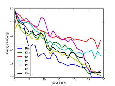
Figure 3: Average similarity of artifact clues in the M57 corpus on the same drive a specified number of days apart in either direction.

 

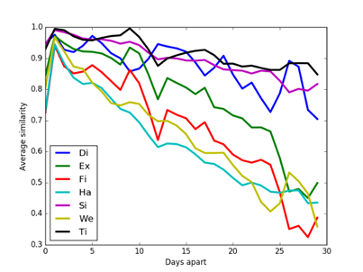
Figure 4: Average similarity of metadata clues in the M57 corpus on the same drive a specified number of days apart.

5.7           Visualizing drive similarities and divergences

Investigators find it helpful to visualize associations of drives.� To do this, we optimized locations in a two-dimensional space to fit distances computed from the similarities and divergences, ignoring similarities under a threshold and divergences over a threshold.� This is an instance of the "embedding problem" in applied mathematics [19] which tries to map a highly dimensional space to fewer dimensions.� The formula with lowest error of fit from similarity to distance from systematic testing on the filtered data in our main corpus was �where D is distance, s is similarity, T is the threshold, and (by experiment) T=0.4.� Similarly, the best formula found for relating divergences to distances was �where d is the divergence for T<3.� Distance errors averaged around 0.4 for both similarities and divergences.� Optimization assigned random locations to start, used an attraction-repulsion algorithm to move locations repeatedly to improve ratios of calculated distances to target distances, then plotted the final locations.� Specifically, the algorithm sought �pairs to minimize this formula over N drives where �is the desired distance between locations i and j:

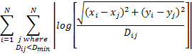
Location optimization used a version of the familiar delta rule for machine learning where changes to the coordinates were proportional to a learning factor (0.1 worked well in these experiments), the distance between the points, and the log ratios shown above.� 20 rounds of optimization were done, followed by rerandomization of the drive locations whose error exceeded a threshold (averaging about 11% of the locations), followed by another 20 rounds of optimization.� Rerandomization gave a second chance to drives that were assigned poor initial locations. ��A minimum-similarity or maximum-divergence threshold can improve optimization speed by excluding weakly associated drive pairs from this optimization.� For instance, setting a threshold of greater than 0.1 for the average clue similarity for a drive reduced the number of drive pairs considered from 177*176/2 = 15,576 to 818 on our Mexican subcorpus.

Figure 5 shows an example visualization of the similarities of the unfiltered hash-value distributions of the 177 Mexican drives, and Figure 6 shows their divergences.� Colors and shapes represent the eight batches in which drives were acquired, which are only weakly correlated with distances though there are several closely related pairs.� A stronger cluster emerges with the divergences.� Since random starting locations are chosen, the display may appear rotated or inverted between two runs on the same input.

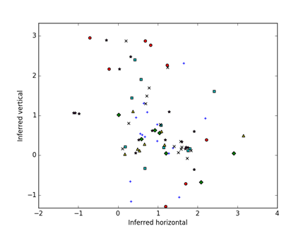
Figure 5: Visualization of the unfiltered Mexican drives based on similarities of the hash-value distributions after optimization; color and shape code the batch out of 8.

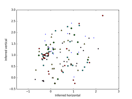
Figure 6: Visualization of the unfiltered Mexican drives based on divergences of the hash-value distributions after optimization; color and shape code the batch out of 8.

 

Figure 7 visualizes the similarities of the distributions of the hash values for the unfiltered M57 files.� Colors and shapes indicate the users here, and their drives are well separated, with some spread involving the early snapshots and two kinds of usage by the user indicated with the green diamonds.

 

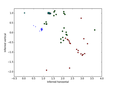
Figure 7: Visualization of the M57 drives based on similarities of the hash-value

�distributions after optimization; color and shape code the simulated users out of 4.

 

Our estimated distances can be used for clustering directly [3].� Graphs can also be built from this data by drawing edges between nodes closer than a threshold distance.� Then a variety of algorithms can analyze the graphs.� For instance, if we set a threshold of 0.5 on the hash-value similarity for the filtered Mexican drives, our software identifies a clique of 24 drives.� Checking the data manually did confirm this was a likely clique and found many similarities between its drives.� Our software also checks for commonalities in each clique; for that example, it noted that the drives in that 24-drive clique are all Windows NT with a hash-value count after filtering from 603 to 1205.

6               Conclusions

This work has shown how computing a few characteristics of drives can be used to infer associations, even if the clues are quite subtle and the drive owners are not aware of it.� Both the cosine similarity and the Kullback-Leibler divergence showed useful results with some differences between them.� Thresholds of significance for similarity were provided on 18 clues for a large corpus.� The clues differ in computational requirements, accuracy, redundancy, and investigative value, however, so we have provided some data to enable an intelligent choice of clues for investigators.� If a quick comparison of drives is desired, comparing email artifacts (sampled at a 0.3 rate) as an indicator of contacts and file extensions (sampled at a 0.03 rate) as an indicator of usage type were adequate.� Hash-value comparisons were time-consuming with few benefits over faster clues, and are thus not recommended.

We also showed the effects of filtering of data before computing similarity, which tended to decrease spurious similarities.� We also discussed the effects of the passage of time on the similarity of images from the same drive, and provided a visualization technique in two dimensions for overall similarities and divergences.� As drive data is increasingly erased or encrypted before forensic analysis, this kind of broad survey will become increasingly difficult to accomplish, so it is valuable to do now.� Our results reflect general principles of what software and people store on drives, and will continue to be valid for a number of years.

7               Acknowledgements

This work was supported by the Naval Research Program at the Naval Postgraduate School under JON W7B27.� The views expressed are those of the author and do not represent the U.S. Government.� Edith Gonzalez-Reynoso and Sandra Falgout helped.

8               References

1.   �Abe, H., and Tsumoto, S., Text categorization with considering temporal patterns of term usages.� Proc. IEEE Intl. Conf. on Data Mining Workshops (2010), pp. 800-807.

2.   Beverly, R., Garfinkel, S., and Cardwell, G., Forensic caving of network packets and associated data structures.� Digital Investigation, Vol. 8, 2011, S78-S89.

3.   �Borgatti, S., and Everett, M. (2000). Models of core/periphery structures. Social Networks 21 (4), 375-395.

4.   �Bulk Extractor 1.5: Digital Corpora: Bulk Extractor [software]. Retrieved on February 6, 2015 from digitalcorpora.org/downloads/bulk_extractor (2013).

5.   �Catanese, S., and Fiumara, G., A visual tool for forensic analysis of mobile phone traffic.� Proc. ACM Workshop on Multimedia in Forensics, Security, and Intelligence, Firenze, Italy, October 2010, pp. 71-76.

6.   �Flaglien, A., Franke, K., and Arnes, A., Identifying malware using cross-evidence correlation.� Proc. IFIP Conf. on Advances in Digital Forensics VIII, AICT 361, 2011, pp. 169-182.

7.   �Forman, G., Eshghi, K., and Chiocchetti, S., Finding similar files in large document repositories.� Proc. 11th ACM SIGKDD Intl. Conf. on Knowledge Discovery in Data Mining, Chicago, IL, US, August 2005, pp. 394-400.

8.   �Garfinkel, S., Forensic feature extraction and cross-drive analysis. Digital Investigation, 3S (September 2006), pp. S71-S81.

9.   �Garfinkel, S., Farrell, P., Roussev, V., Dinolt, G., Bringing science to digital forensics with standardized forensic corpora. Digital Investigation 6 (August 2009), pp. S2-S11.

10. Jones, A., Valli, C., Dardick, C., Sutherland, I., Dabibi, G., and Davies, G., The 2009 analysis of information remaining on disks offered for sale on the second hand market.� The Journal of Digital Forensics, Security and Law, Vol. 5, No. 4 (2010), Article 3.

11. Mohammed, H., Clarke, N., and Li, F., An automated approach for digital forensic analysis of heterogeneous big data. The Journal of Digital Forensics, Security and Law, Vol. 11, No. 2, 2016, Article 9.

12. Nassif, L., and Hruschka, E., Document clustering for forensic analysis: An approach for improving computer inspection.� IEEE Transactions on Information Forensics and Security, 8 (1) (January 2013), pp. 46-54.

13. Pateriya, P., Lakshmi, and Raj, G., A pragmatic validation of stylometric techniques using BPA.� Proc. Intl. Conf. on The Next Generation Information Technology: Confluence, 2014, pp. 124-131

14. Patterson, J., and Hargreaves, C., The potential for cross-drive analysis using automated digital forensic timelines.� Proc. 6th Int. Conf. on Cybercrime Forensics and Training, Canterbury, NZ, October 2012.

15. Raghavan, S., Clark, A., and Mohay, G., FIA: An open forensic integration architecture for composing digital evidence.� Proc. Intl. Conf. of Forensics in Telecommunications, Information and Multimedia, 2009, pp. 83-94.

16. Rowe, N., Identifying forensically uninteresting files in a large corpus.� EAI Endorsed Transactions on Security and Safety, Vol. 16, No. 7 (2016), article e2.

17. Rowe, N., Finding and rating personal names on drives for forensic needs, Proc. 9th EAI International Conference on Digital Forensics and Computer Crime, Prague, Czech Republic, October 2017.

18. Rowe, N., Schwamm, R., McCarrin, M., Gera, R., Making sense of email addresses on drives. Journal of Digital Forensics, Security, and Law, Vol. 11, No. 2, 2016, pp. 153-173.

19. Sippl, M., and Scheraga, H., Solution of the embedding problem and decomposition of symmetric matrices.� Proc. National Academy of Sciences, USA, Vol. 82, pp. 2197-2201, April 1985.

20. Sun, M., Xu, G., Zhang, J., and Kim, D., Tracking you through DNS traffic: Linking user sessions by clustering with Dirichlet mixture model.� Proc. 20th ACM Intl. Conf. on Modeling, Analysis, and Simulation of Wireless and Mobile Systems, Miami, FL, US, November 2017, pp. 303-310.

21. Tabish, S., Shafiq, M., Farooq, M., Malware detection using statistical analysis of byte-level file content.� Proc. ACM Workshop on Cybersecurity and Intelligence, Paris, France, June 2009, pp. 23-31.

22. Van Bruaene, J, Large scale cross-drive correlation of digital media.� M.S. thesis, U.S. Naval Postgraduate School, March 2016,

23. Whissell, J., and Clarke, C., Effective measures for inter-document similarity.� Proc. 22nd ACM Intl. Conf. on Information and Knowledge Management, 2013, pp. 1361-1370.

24. Woods, K., Lee, C., Garfinkel, S., Dittrich, D., Russell, A., and Kearton, K., Creating realistic corpora for security and forensic education.� Proc. ADFSL Conference on Digital Forensics, Security, and Law, 2011, pp. 123-134.

25. Zhao, S., Yu, L., And Cheng, B., Probabilistic community using link and content for social networks.� IEEE Access, Vol. PP, No. 99 (November 2017).

26. Zhou, D., Manavoglu, E., Li, J., Giles, C., and Zha, H., Probabilistic models for discovering e-communities.� Proc. of WWW Conference, May 23-26, 2006, Edinburgh, Scotland, pp. 173-182.